HF Receiver Principles
HF Receiver Principles. Noise and Dynamic Range Jamie Hall WB4YDL. April 26, 2012. Reelfoot Amateur Radio Club. Receiver Sensitivity Limitations. Define Ant Noise Factor Noise Temp F(x) of graph Frequency Ant Noise Factor Noise Temp. Overview Linear except Daytime atmosphere.


HF Receiver Principles
E N D
Presentation Transcript
HF Receiver Principles Noise and Dynamic Range Jamie Hall WB4YDL April 26, 2012 Reelfoot Amateur Radio Club
Receiver Sensitivity Limitations Define Ant Noise Factor Noise Temp F(x) of graph Frequency Ant Noise Factor Noise Temp. Overview Linear except Daytime atmosphere
Understanding Logarithms • A logarithm is simply an exponent. • Example: given a base of 2 and an exponent of 3 we have 2³ = 8. • Inversely: given a base of 2 and power 8, (2ⁿ = 8), then what is the exponent that will produce 8 ? • That exponent is called the logarithm. • We say the exponent 3 is the logarithm of 8 with base 2. • 3 is the exponent to which 2 must be raised to produce 8.
Understanding Logarithms (con’t) • Common logarithms use base 10 and are used in fields such as engineering, physics, chemistry, and economics. • Since 10³ = 1000, then log 1000 = 3. • 3 is the exponent to which 10 must be raised to produce 1000. • Using logarithms greatly simplifies talking about differences in very large and very small numbers. • Important logarithm rule: • log (x/y) = log x – log y
How to find logarithms Calculator – use base 10, not ln (natural) Table of logarithms Slide rule. What’s that? Basics of determining the Characteristic and mantissa
Using Decibels in Ham Radio Using dB allows us to talk about very large differences in power or voltage levels with numbers that are easy to comprehend. Example: The maximum power output of a transmitter in the USA is 1500 watts and the noise floor of a modern receiver is 0.04 microvolts. The received power at this voltage level into 50 ohms (E²/R) is 0.000000000000000032 watts or 3.2 x 10⁻¹⁷. This is not easy to deal with ! We refer to power levels as dB above or below 1 miliwatt in a 50 ohm system and call the result dBm. Thus 1 milliwatt is 0 dBm. 1500 watts in dBm = 10 log (1500 / .001) = +62 dBm 3 x 10-17 watts in dBm = 10 log (3 x 10-17 / .001) = -135 dBm This is much easier to comprehend and deal with. Question: How many dBm does a 100 watt transmitter produce ?
Dynamic Range • In general, DR is the ratio (or difference in dB) between the weakest signal a system can handle and the strongest signal that same system can handle simultaneously. • Example: The normal human ear can detect a 1 kHz sound wave at a level of 10-12 watts/m² while the upper limit is about 1 watt/m², where pain is felt. The dynamic range of our ears is thus about 120 dB. • Example: Our eyes can detect the light from a star in a dark sky when about 10 photons per second reach the retina, which is about 10-13 watts/m². The Sun with its 300 watts/m², does not damage our eyes unless we look straight into it. • The baseball outfielder who drops a fly ball certainly knows about the blocking effects of the Sun. He employs an attenuator (sunglasses) to reduce the interference, but this may in fact put the desired signal (the baseball) below his noise floor. In radio, the attenuator would be a front-end AGC.
Blocking Dynamic Range BDR is the difference in dB between minimum discernible signal (MDS) and an off-channel signal that causes 1 dB of compression in the receiver.
Sensitivity and Blocking • Blocking happens when a large off channel signal causes the front-end RF amplifier to be driven to its compression point. • As a result all other signals are lost (blocked). • This condition is frequently called de-sensing—the sensitivity of the receiver is reduced. • Blocking is generally specified as the level of the unwanted signal at a given offset. • Original testing used a wide offset—typically 20 kHz. More recently, recognizing our crowded band conditions and the narrow spacing of CW and other digital modes, most testing today is done with close spacing of 2 kHz.
IMD 2 kHz Away IMD 20 kHz Away 15 kHz Wide 15 kHz Wide First IF Filter at 70.455 MHz First IF Filter at 70.455 MHz Wide & Close Dynamic Range 20 kHz Spacing 2 kHz Spacing
Nonlinearity and Intermodulation Distortion • Nonlinearity in RF and IF circuits leads to two undesirable outcomes: harmonics and intermodulation distortion. • Harmonics in and of themselves are not particularly troublesome. • For example, if we are listening to a QSO on 7.230 MHz, the second harmonic, 14.460 MHz is well outside the RF passband. • However, when the harmonics mix with each other and other signals in the circuit, undesirable and troublesome intermodulation products can occur.
Intermodulation Distortion (IMD) RCV INPUT FILTER
Intermodulation Distortion Products: An Example f1 f2 2f1- f2 2f2- f1 3f1- 2f2 3f2- 2f1
Third Order Intermodulation Products • The 3rd order products will be the largest (loudest) of the intermodulation products. • As a general rule, the 3rd order products will increase (grow) 3-times faster than the fundamental signal (the signal of interest).
ARRL Receiver Test:Measured Response of the Signal of Interest
ARRL Receiver Test:Extrapolated Linear Region of the Measured Response of the Signal of Interest
ARRL Receiver Test:Extrapolated Linear Region of theMeasured Response of the IMD Product
The 3rd order intercept point (IP3): A Measure of Merit Our graph illustrates that the 3rd order intercept point is defined by the intersection of two hypothetical lines. Each line is an extension of a linear gain figure: first of the signal of interest; and second, of the 3rd order intermodulation distortion product—from which IP3 gets its name. You will note that the larger the value of IP3, the less likely the receiver will be adversely affected by 3rd order intermodulation products.
ARRL Receiver Test:Extrapolated Linear Region of theMeasured Response of the IMD Product IMD Dynamic Range
Summary Rx sensitivity limitations Antenna noise factor, frequency, noise temp Logs & decibels to manage references Dynamic range, BDR, Sensitivity & blocking IMD, 3rd order IMD Examples of receiver tests : Sensitivity [(S+N)/N] and MDS measurement and S-meter calibration