Developing ICPRB’s Potomac Watershed Model using Soil & Water Assessment Tool
210 likes | 459 Vues
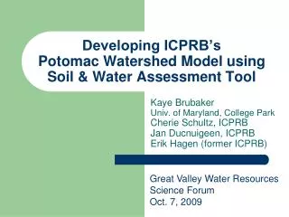
Developing ICPRB’s Potomac Watershed Model using Soil & Water Assessment Tool. Kaye Brubaker Univ. of Maryland, College Park Cherie Schultz, ICPRB Jan Ducnuigeen, ICPRB Erik Hagen (former ICPRB). Great Valley Water Resources Science Forum Oct. 7, 2009. Why a Potomac Watershed Model?.

Developing ICPRB’s Potomac Watershed Model using Soil & Water Assessment Tool
E N D
Presentation Transcript
Developing ICPRB’sPotomac Watershed Model usingSoil & Water Assessment Tool Kaye Brubaker Univ. of Maryland, College Park Cherie Schultz, ICPRB Jan Ducnuigeen, ICPRB Erik Hagen (former ICPRB) Great Valley Water Resources Science Forum Oct. 7, 2009
Why a Potomac Watershed Model? • Understand the physical processes associated with variability in water supply • Understand the effects of human activities on water supply • Predict potential effects of future climatic and land use changes • Allow more accurate assessments of • drought risk • need for resource development • Implications for management
Why SWAT? (Soil & Water Assessment Tool) • Ease of use, Portability • Free of charge (USDA Agricultural Research Service) • Model set-up – GIS interface (ArcSWAT) • Changes to land use easy to implement • Once built, model runs at “Command” prompt • Longevity • Future investigators can learn the model and keep it updated • Modeling system has a long history & should be supported in the future • Spatio-temporal formulation • Considers spatial pattern on the landscape • Can simulate long periods using continuous time
Shenandoah Model: 3 HUCs
Transpiration Evaporation Precipitation V e g Direct Runoff Surface Interflow Soil Layer Stream Baseflow Shallow Aquifer Deep Aquifer
ptf # .gw file Subbasin:12 HRU:5 Luse:FRSD Soil: VA005 Slope: 0-10 12/21/2007 12:00:00 AM ARCGIS-SWAT interface MAVZ 1000.0000 | SHALLST : Initial depth of water in the shallow aquifer [mm] 1000.0000 | DEEPST : Initial depth of water in the deep aquifer [mm] #gdva005# | GW_DELAY : Groundwater delay [days] #ava005# | ALPHA_BF : BAseflow alpha factor [days] 1000.0000 | GWQMN : Threshold depth of water in the shallow aquifer required for return flow to occur [mm] #rvva005# | GW_REVAP : Groundwater "revap" coefficient #revapmn# | REVAPMN: Threshold depth of water in the shallow aquifer for "revap" to occur [mm] 0.0000 | RCHRG_DP : Deep aquifer percolation fraction 1.0000 | GWHT : Initial groundwater height [m] 0.0030 | GW_SPYLD : Specific yield of the shallow aquifer [m3/m3] 0.0000 | SHALLST_N : Initial concentration of nitrate in shallow aquifer [mg N/l] 0.0000 | GWSOLP : Concentration of soluble phosphorus in groundwater contribution to streamflow from subbasin [mg P/l] 0.0000 | HLIFE_NGW : Half-life of nitrate in the shallow aquifer [days] #bva005# | B_BF: Baseflow "b" exponent
ptf # .mgt file Subbasin:12 HRU:5 Luse:FRSD Soil: VA005 Slope: 0-10 11/30/2007 12:00:00 AM ARCGIS-SWAT2003 interface MAVZ 0 | NMGT:Management code Initial Plant Growth Parameters 0 | IGRO: Land cover status: 0-none growing; 1-growing 0 | PLANT_ID: Land cover ID number (IGRO = 1) 0.00 | LAI_INIT: Initial leaf are index (IGRO = 1) 0.00 | BIO_INIT: Initial biomass (kg/ha) (IGRO = 1) 0.00 | PHU_PLT: Number of heat units to bring plant to maturity (IGRO = 1) General Management Parameters 0.20 | BIOMIX: Biological mixing efficiency 72.00 | CN2: Initial SCS CN II value 1.00 | USLE_P: USLE support practice factor 0.00 | BIO_MIN: Minimum biomass for grazing (kg/ha) 0.000 | FILTERW: width of edge of field filter strip (m) Urban Management Parameters 0 | IURBAN: urban simulation code, 0-none, 1-USGS, 2-buildup/washoff 0 | URBLU: urban land type Irrigation Management Parameters 0 | IRRSC: irrigation code 0 | IRRNO: irrigation source location 0.000 | FLOWMIN: min in-stream flow for irr diversions (m^3/s) 0.000 | DIVMAX: max irrigation diversion from reach (+mm/-10^4m^3) 0.000 | FLOWFR: : fraction of flow allowed to be pulled for irr Tile Drain Management Parameters 0.000 | DDRAIN: depth to subsurface tile drain (mm) 0.000 | TDRAIN: time to drain soil to field capacity (hr) 0.000 | GDRAIN: drain tile lag time (hr) Management Operations: 1 | NROT: number of years of rotation Operation Schedule: 0.150 1 7 3600.00000 0.00 0.00000 0.00 0.00 #c5d# 0.200 6 108 #c5g# 1.200 5 #c5d# 0
Linear Reservoir Model Where S = Storage Q = Discharge (volume/day) K = Recession coefficient (days) Note that, for pure recession, This has the solution Which plots as a straight line on a semi-log graph
one log cycle recession index, K [days]
Advantages of Linear Model • Reasonable physical concept – outflow is greatest when reservoir is full • Closed-form solution • A parameter with dimension of time – easy to understand
But is it realistic for GW flow? • Observations indicate that real baseflow aquifers (e.g., in the Shenandoah Valley) don’t behave as we would like! • Can show with physical arguments (Wittenberg 1999) that, with typical assumptions for unconfined aquifers, a better assumption would be
Wittenberg (1999) Model • Analyzed rivers in Germany and found a more general result Found values of b between 0 and 1.1, with a mean value of 0.49. (Set b = 1 to get the linear model.)
Incorporation into SWAT • Wrote new groundwater module for SWAT • Calculates groundwater flow as an explicit function of state variable for GW storage where S is shallow aquifer storage [L] Smin is the minimum storage for GW flow [L] a is a scale parameter [weird dimensions] b is a coefficient [dimensionless]
Shenandoah Model • 3 HUCs • 28 Subbasins • 489 HRUs
Preliminary Application Not Calibrated Shenandoah at Millville
Calibration Principles • physical fidelity • parsimony • sensitivity, and • repeatability.