Boosted Regression Trees A method to explore biology-environment relationships
170 likes | 292 Vues
This study by Sophie Mormede and Matt Pinkerton at the National Institute of Water and Atmospheric Research presents the application of Boosted Regression Trees (BRT) to understand ecological dependencies and habitat preferences within the Ross Sea. BRT is utilized to predict distributions of toothfish and bycatch species, assess bioregionalization layers, inform conservation planning, and evaluate species distribution changes due to climate scenarios. The advantages of BRT over traditional models include resilience to missing data, handling of non-normal distributions, and a capacity for complex interactions, while also addressing challenges such as overfitting.

Boosted Regression Trees A method to explore biology-environment relationships
E N D
Presentation Transcript
Boosted Regression TreesA method to explore biology-environment relationships Sophie Mormede, Matt Pinkerton National Institute of Water and Atmospheric Research, Wellington, NZMay 2010
Two main uses of BRT • to investigate the ecological dependence of a species on the environment • to determine "habitat preference" in order to extrapolate patchy biological data to a larger domain
An example • WHAT: Predict toothfish and bycatch species distributions over the Ross Sea (88.1 & 882A–B) • WHY: • layers for bioregionalisation • input to systematic conservation planning • to investigate overlap of TOA and prey species • to consider potential changes in species distribution under climate change scenarios • to help in estimating biomass from the small number of research trawls (WGR) • HOW: GLM / GAM (not very satisfactory), BRT, General Dissimilarity Matrices, …
Project outcomes so far • Predictions seem to make sense, and confidence intervals • Quality of depth data critical (use gebco08, modified with fishing depth) • Still need to validate models on a different area (882E?, Kerguelen?)
BRT – what is it all about then? • Regression Tree: • Recursive binary splits • Stopping criterion • Allows interactions natively if wanted (tree complexity) • Boosting = forward stagewisemodel fitting: • A truncated tree (1-10 splits) • Computed the fitted values and residuals • Fit and add a new tree to the residuals, repeating many times (number of trees > 1000)
More about BRT • Boosting with stochasticity: • At each step a proportion of dataset is randomly selected (bag fraction) to be fitted to, improves model performance • Cross validation (CV): • To avoid overfitting, test model on withheld parts of the data – also estimates overfitting • You can bootstrap BRTs (I used 1000 bootstraps)
Pros of BRT • Copes with NAs, • Copes with non normally-distributed environmental variables (no transforms), • Copes with outliers • Allows multiple levels of interactions • Unlikely to overfit as much as GLM, quantifies • 20-30% improvement of fits compared with GLM / GAM • Runs on R
Cons of BRT • Cons of BRT • Does not give smooth / monotonic responses • Still some overfitting – need to be careful • Slow when using bootstrapping • Cons of any prediction method • Only as good as the environmental layers • Predict only in the domain we have data for (need to mask other areas)
BRT process • Optimise BRT setup (which variables, how many interactions, based on deviance) • Run full models and bootstraps • Run reduced models with only variables that were significant • Bootstrap predictions based on reduced model, and calculate CI • Plot
Back to the example environmental variables we used • Bathymetry (Gebco 2008, modified for fishing depth) • Chlorophyll A summer (remote sensing) • Ice15 and ice85 (satellite data) – not used • Rugosity (Gebco08) • Near bottom current speed, temperature and salinity (HIGEM circulation model) • Use only variables that make biological sense!
Predictor variables • For each species, predict proportion of hooks that caught a fish • Akin to binomial per hook • Transform to normalise data • Y = arcsin [ sqrt (fish per hook) ] • Predict with BRT using Gaussian link • Also predict binomial for all but toothfish (only 5% null catch) • Could also do fish per line
CPR database BRT Other example – Oithona similisPinkerton et al. (2010) Oithona similis The most abundant animal in the world?
Others methods to considerGeneral Dissimilarity Modelling • General Dissimilarity Modelling: Multivariate response variable • Pros • predict communities based on environmental variables (multiple species analysed) • Classification part of the process • Cons • No bootstrapping • How many species??
Classification • Classifications (clusters): separates areas based on layers (environment, biology etc) • Options • Use biology layers from BRT? • Use environmental layers too? (double-dipping?) • Use GDM directly for predictions and classifications? • Number of classes…