2.2
2.2. Organizing Quantitative Data. Data. Consider the following data We would like to compute the frequencies and the relative frequencies. Show the Frequency and Rel. Frequency. Histogram.

2.2
E N D
Presentation Transcript
2.2 Organizing Quantitative Data
Data • Consider the following data • We would like to compute the frequencies and the relative frequencies
Histogram • Discrete quantitative data can be presented in bar graphs in several of the same ways as qualitative data • We use the discrete values instead of the category names • We arrange the values in ascending order • For discrete data, these are called histograms
Histograms • Example of histograms for discrete data • Frequencies • Relative frequencies • Use calculator • Enter values from table into a list • Plot values and change to histogram
Calculator Practice • Making a histogram
Classes • Continuous data cannot be put directly into frequency tables since they do not have any obvious categories • Categories are created using classes, or intervals of numbers • The continuous data is then put into the classes
Classes • For ages of adults, a possible set of classes is 20 – 29 30 – 39 40 – 49 50 – 59 60 and older • For the class 30 – 39 • 30 is the lowerclasslimit • 39 is the upperclasslimit
Class Width • The classwidth is the difference between the upper class limit and the lower class limit • For the class 30 – 39, the class width is 40 – 30 = 10 • Why isn’t the class width 39 – 30 = 9? • The class 30 – 39 years old actually is 30 years to 39 years 364 days old … or 30 years to just less than 40 years old • The class width is 10 years, all adults in their 30’s
Open Ended Classes • All the classes (20 – 29, 30 – 39, 40 – 49, 50 – 59) all have the same widths, except for the last class • The class “60 and above” is an open-endedclass because it has no upper limit • Classes with no lower limits are also called open-ended classes
The classes and the number of values in each can be put into a frequency table • How many people are between 30 and 39 years old?
Stem-and-Leaf Plot • A stem-and-leafplot is a different way to represent data that is similar to a histogram • To draw a stem-and-leaf plot, each data value must be broken up into two components • The stem consists of all the digits except for the right most one • The leaf consists of the right most digit • For the number 173, for example, the stem would be “17” and the leaf would be “3”
Stem-and-Leaf Plots • Modifications to stem-and-leaf plots • Sometimes there are too many values with the same stem … we would need to split the stems (such as having 10-14 in one stem and 15-19 in another) • If we wanted to compare two sets of data, we could draw two stem-and-leaf plots using the same stem, with leaves going left (for one set of data) and right (for the other set)
Create a Stem-and-leaf plot • Birth DATE for students in this class
Dot Plot • A dotplot is a graph where a dot is placed over the observation each time it is observed • Not extremely useful but help give us a quick view of distribution • Make a Dot Plot with the Birthday MONTH
Distribution Shape • A useful way to describe a variable is by the shape of its distribution • Some common distribution shapes are • Uniform • Bell-shaped (or normal) • Skewed right • Skewed left
Uniform • A variable has a uniform distribution when • Each of the values tends to occur with the same frequency • The histogram looks flat
Bell-Shaped • A variable has a bell-shaped distribution when • Most of the values fall in the middle • The frequencies tail off to the left and to the right • It is symmetric
Skewed Right • A variable has a skewedright distribution when • The distribution is not symmetric • The tail to the right is longer than the tail to the left • The arrow from the middle to the long tail points right
Skewed Left • A variable has a skewedleft distribution when • The distribution is not symmetric • The tail to the left is longer than the tail to the right • The arrow from the middle to the long tail points left
Time-Series Graph • The following is an example of a time-series graph • The horizontal axis shows the passage of time