A Prototype Example: The Galaxy Linear Programming Model
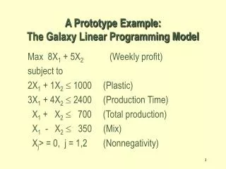
A Prototype Example: The Galaxy Linear Programming Model. Max 8X 1 + 5X 2 (Weekly profit) subject to 2X 1 + 1X 2 £ 1000 (Plastic) 3X 1 + 4X 2 £ 2400 (Production Time) X 1 + X 2 £ 700 (Total production) X 1 - X 2 £ 350 (Mix)

A Prototype Example: The Galaxy Linear Programming Model
E N D
Presentation Transcript
A Prototype Example: The Galaxy Linear Programming Model Max 8X1 + 5X2 (Weekly profit) subject to 2X1 + 1X2£ 1000 (Plastic) 3X1 + 4X2£ 2400 (Production Time) X1 + X2£ 700 (Total production) X1 - X2£ 350 (Mix) Xj> = 0, j = 1,2 (Nonnegativity)
The Graphical Analysis of Linear Programming The set of all points that satisfy all the constraints of the model is called a FEASIBLE REGION
Using a graphical presentation we can represent all the constraints, the objective function, and the three types of feasible points.
Graphical Analysis – the Feasible Region The non-negativity constraints X2 X1
The Plastic constraint 2X1+X2 = 1000 Graphical Analysis – the Feasible Region X2 1000 700 Total production constraint: X1+X2 =700 (redundant) 500 Infeasible Feasible Production Time 3X1+4X2 = 2400 X1 500 700
Graphical Analysis – the Feasible Region X2 The Plastic constraint 2X1+X2 = 1000 1000 700 Total production constraint: X1+X2 = 700 (redundant) 500 Infeasible Production mix constraint: X1-X2 =350 Feasible Production Time 3X1+4X2= 2400 X1 500 700 • Boundary points. Extreme points. • Interior points. • There are three types of feasible points
The search for an optimal solution Start at some arbitrary profit, say profit = $2,000... X2 Then increase the profit, if possible... 1000 ...and continue until it becomes infeasible 700 Profit =$4360 500 X1 500
Summary of the optimal solution Space Rays = 320 dozen Zappers = 360 dozen Profit = $4360 • This solution utilizes all the plastic and all the production hours. • Total production is only 680 (not 700). • Space Rays production exceeds Zappers production by only 40 dozens.
Main Result: Extreme points and optimal solutions • If a linear programming problem has an optimal solution, an extreme point is optimal.
Computer Solution of Linear Programs With Any Number of Decision Variables • Linear programming software packages solve large linear models i.e. many decision variables and many constraints. • Graphical method is limited to 2-decision variable LP problems, however, LP software packages use the Main Result of graphical method, called the Simplex algorithm. • The input to any package includes: • The objective function criterion (Max or Min). • The type of each constraint: . • The actual coefficients for the problem.