Case-control association techniques in genetic studies
Case-control association techniques in genetic studies. March 10, 2011. Karen Curtin, Ph.D. Division of Genetic Epidemiology and HCI Pedigree & Population Resource (PPR). Presentation outline. Background (genetics concepts). Basic case-control association.

Case-control association techniques in genetic studies
E N D
Presentation Transcript
Case-control association techniques in genetic studies March 10, 2011 Karen Curtin, Ph.D. Division of Genetic Epidemiology and HCI Pedigree & Population Resource (PPR)
Presentation outline • Background (genetics concepts) • Basic case-control association • Complex case-control association • Genome-wide association
The Human Genome: 6 billion DNA bases(Adenine, Cytosine, Guanine, or Thymine) License: Creative Commons Attribution 2.0
…AGCCAAACTGAATTC… …AGCCAAATTGGATTC… At any locus (position on a chromosome): Read across both chromosomes Genotype CT CA T G Read along a chromosome Haplotypes: C-A and T-G Genotype and Haplotype If allele T can predict allele G, two alleles are in Linkage Disequilibrium (LD)
90% of genomic variants are SNPs Single Nucleotide Polymorphsim Two alternate forms (alleles) that differ in sequence at one point in a DNA segment Source: David Hall, Creative Commons Attribution 2.5 license
Genetic variants: Germline v Somatic • Germline variant/mutations • Inherited/In-born mutation • In all cells • In particular, in germline haploid cells • Heritable • Cell division - meiosis • Somatic variants/mutations • Acquired mutation • Only in an isolated number of cells (tumor site) • Generally not heritable • Cell division - mitosis
Hereditary mutation - meiosis Parent germ cells Daughter cells HAPLOID X New zygotes DIPLOID
Presentation outline • Background (genetics concepts) • Basic case-control association • Complex case-control association • Genome-wide association
Genetic variants in association studies Association: two characteristics (disease& genetic variant) occur more often together than expected by chance • Direct Association / Causal Functional variant Disease • Functional variant is involved in disease • Functional variant is associated with the disease • Indirect Association Genetic variant Functional variant Disease • Genetic variant (SNP) is associated/correlated with underlying functional variant • Functional variant is involved in disease • Genetic variant (marker) is associated with disease (initial step.. Ultimate goal is to discover causal variant)
Genetic association study Designs • Observational • Exposure variables • Genetic variants • Environmental factors • Classical association study designs • Unit of interest is an individual • Cohort study (cross-sectional or longitudinal) • Case-control study • Family-based association study • Unit of interest is a family unit
Case-Control Study • Sample individuals based on to disease status and without knowledge of exposure status (e.g. genotype) • CASES (with disease) • CONTROLS (no disease) • Usually balanced design (#cases = #controls) • Retrospective • Neither prevalence nor incidence can be estimated
Types of Case-Control Study • Population-based • Risk estimates can be extrapolated to the source population • Could be nested in a cohort study • Selected sampling • Increases power to detect associations • Antoniou & Easton (2003) • Tests of independence are valid • True positive risks are exaggerated • Can not be extrapolated
Case-Control: Population-based • Source population • All individuals satisfying predefined criteria • Source cohort • A group that is ‘representative’ of the source population • CASES and CONTROLS occur in relation to population prevalence • CASES • Cases selected are ‘representative’ of cases in the source cohort • In particular, in terms of the exposure variables • CONTROLS • Controls selected are ‘representative’ of controls in the source cohort • In particular, in terms of the exposure variables • Odds Ratio (estimate of the relative risk) can be extrapolated back to the source population • Population Attributable Risk (PAR)
Case-Control: Selected Sampling • Source population • All individuals satisfying predefined criteria • Source cohort • A group that is ‘representative’ of the source population • CASES and CONTROLS occur in relation to population prevalence • CASES • Cases selected are in effect selectively sampled from cases in source cohort • Family history of disease, severe disease, early onset,… • CONTROLS • Cases selected are in effect selectively sampled from controls in source cohort • Screened negative, no family history,… • Association analyses are still valid and power may be increased • BUT… • Odds Ratio (estimate of the relative risk) can not be extrapolated back to the source population
Case-Control Study: Odds Ratio Exposure Yes No Disease Cases (Yes) a b Controls(No) c d Odds Ratio (OR) = a / b = a × d c / d b × c H0: OR = 1 same risk (no association) OR > 1 indicates increased risk OR < 1 indicates decreased risk (protective)
95% confidence intervals for the Odds Ratio Lower and Upper bounds for the risk estimates. Two common methods: • eln(OR) – 1.96se(ln(OR)), eln(OR) + 1.96se(ln(OR)) where se(ln(OR)) = 1/a+1/b+1/c+1/d 2) OR1-1.96/, OR1+1.96/
chi-square test Compares observed values (O) with those expected under independence between rows and columns Expected (E) = row total column total N chi-square statistic, with (rows-1) (columns-1) degrees of freedom 2 = (O – E)2 ~ 2(rows-1) (columns-1) E
Test for Non-independence H0: Disease and exposure (genotype) are independent chi-square tests: contingency tables 2×3 genotype table (2 df) 2×2 grouped genotype table (1 df) • Dominant or recessive 2×3 ‘dose-dependent’ table • Armitage test for trend (1 df) 2×2 allele table (1 df)
Modeling genetic exposures • Exposure = genotype • Single variant with 2 alleles (SNP) • Three genotypes: CC, CT, TT • 23 contingency table • Chi-sq 2df • Chi-sq 1df (impose a linear dependency between columns) CC CT TT Controls Cases
Mode of Expression / Inheritance • Let allele C be disease causing • Examples of modes of expression are: • Dominant TT TCCC • Individuals heterozygous or homozygous for the C allele gives rise to the disease • Recessive TT TC CC • Only homozygous individuals for the C allele results in disease • Codominant TT TCCC • All three genotypes can be distinguished phenotypically • ‘Additive’ model – TC has r-fold risk, CChas 2r effect
chi-square test CC CT TT Totals Chi-stat= (120-120)2 + (40-50)2 + (20-30)2 +(120-120)2 +(60-50)2 + (40-30)2 120 50 30 120 50 30 Chi-statistic = 10.67 p-value=0.0048 (for a chi-square distribution with 2 df) Controls 200 120 50 30 Cases 200 120 50 30 400 240 100 60 Totals
Genotypic relative risk • Assess risk (OR) for each genotype relative to the homozygous common genotype ORhet = a × e ORhzv = a × f CT vs. CC b × d TT vs. CC c × d Genotype (exposure) CC CT TT Controls Cases
chi-square test / genotypic relative risk CC CT TT Totals Chi-stat= (120-120)2 + (40-50)2 + (20-30)2 +(120-120)2 +(60-50)2 + (40-30)2 120 50 30 120 50 30 Chi-statistic = 10.67 p-value=0.0048 (for a chi-square distribution with 2 df) OR het CT vs. CC = 1.5 OR hzv TT vs. CC = 2.0 Controls 200 120 50 30 Cases 200 120 50 30 400 240 100 60 Totals
Test for Non-independence H0: Disease and exposure (genotype) are independent chi-square tests: contingency tables 2×3 genotype table (2 df) 2×2 grouped genotype table (1 df) • Dominant or recessive 2×3 ‘dose-dependent’ table • Armitage test for trend (1 df) 2×2 allele table (1 df)
Dominant model for exposure Exposure = CT&TT genotypes - 22 test with 1 df ORdom = a × (e+f) = 1.67 d × (b+c) Genotype CC CT TT (b+c)= Controls Cases (e+f)=100
Recessive model for exposure Exposure = TT genotype (vs. CC&CT) - 22 test w/1 df ORrec = (a+b) × f = 1.78 (d+e) × c Genotype CC CTTT Controls (a+b)=160 Cases (d+e)=180
Test for Non-independence H0: Disease and exposure (genotype) are independent chi-square tests: contingency tables 2×3 genotype table (2 df) 2×2 grouped genotype table (1 df) • Dominant or recessive 2×3 ‘dose-dependent’ table • Armitage’s trend test (1 df) 2×2 allele table (1 df)
Armitage Trend Test (23 with 1df) Assess departures from a fitted trend CC (x1=0) CT (x2=1) TT (x3=2) R Controls Cases n1 n2 n3 N
Example – genotypic relative risk and trend test Shephard et al. Cancer Res 2009
Test for Non-independence H0: Disease and exposure (genotype) are independent chi-square tests: contingency tables 2×3 genotype table (2 df) 2×2 grouped genotype table (1 df) • Dominant or recessive 2×3 ‘dose-dependent’ table • Armitage’s trend test (1 df) 2×2 allelic table (1 df)
Allelic Test • Exposure = Allele (T vs. C) • 2 x 2 table (1 df) for a single SNP • Count every allele (2 per person) • Doubles the sample size ORallele = (2a+b)×(2f+e) (2c+b)×(2d+e) Allele C T Controls OR = 1.633 T vs. C allele Cases
Example – allelic association 11 12 22 11 12 22 Xue et al. Arch Oral Bio 2009
More flexible techniques • If other factors may have an effect on disease status (affected/unaffected, case/control) • We want to account for these as covariates • We want to adjust for matching variables (age, sex, etc.) • Logistic regression • Logistic transformation (logit) • ln(p/(1-p)) = + 1x1 + 2x2 + …. • Coefficients and ’s are estimated using maximum likelihood estimation (MLE) • Test H0: =0 against H1: = using a likelihood ratio test (LRT) • Must decide on how to model the genetic exposure • genotype categories (i.e. CC, CT,TT), dominant, recessive, additive (allele dose).. ~ ~ ^
Example of logistic regression model with genetic exposure and covariates Slattery et al. IJC 2010
Assumptions for Validity • Independence of all individuals • Independent and identically distributed (iid) • Reasonable sample sizes • Contingency tables • Expected values all > 1 and 80% > 5 • Logistic regression • Minimum of 15-20 individuals per group • If violated • Simulate the null distribution for testing • Permutation test • e.g. Fishers exact test is an exhaustive permutation test • Monte Carlo simulation
Presentation outline • Background (genetics concepts) • Basic case-control association • Complex case-control association • Genome-wide association
Performing haplotype analyses • Single locus • We observe genotypes, so testing is straight-forward counting into a contingency table CC CT TT Controls Cases
Performing haplotype analyses • Multi-locus • Haplotypes are not directly observed • But can be estimated (EM/Bayesian…) • For some individuals, their haplotype pair can be inferred unambiguously • For many individuals they can not • “Phase uncertainty” • All analyses of haplotypes must take into account the phase uncertainty in the data • Otherwise, increase in type 1 errors
Haplotypes / Genotypes Two-locus Haplotypes: The haplotype pair must be: C-G and C-G UNAMBIGUOUS …AGCTAAACTGGATT… …AGCCAAACTGGATT… CG CG
Estimating haplotypes Genotypes Locus 1 Locus 2 Haplotypes CCGGC-G&C-G CCGAC-G&C-A CCAAC-A&C-A CTGGC-G&T-G CTGA?(C-G&T-A) or (C-A&T-G)? CTAAC-A&T-A TTGGT-G&T-G TTGAT-G&G-A TTAAT-A&T-A
Estimating haplotypes • Expectation-maximization (EM) algorithm • SNPHAP (Johnson et al 2001) • GCHap (Thomas 2003) • Bayesian MCMC approach • PHASE (Stephens et al 2001) • Both approaches assume independent individuals • Use to estimate • Population haplotype frequencies estimated from a set of individuals • Most likely haplotype pair for each individual
Traditional methods for phase uncertainty • Likelihood based approach • Each individual can have multiple different haplotype pairs that are consistent with the genotype data • Some pairs of haplotypes are more or less likely than others • Each pair is given a weight • All possible haplotype pairs are considered in the case-control analysis • weighted by their probabilities
Simulation methods for phase uncertainty • Sample over the observed data • Instead of weighting all the possible haplotype pairs for every individual and incorporating all at once into the analysis • Sample one pair of each individual • Randomly and in proportion to the weights, select a haplotype pair for each individual • Perform the analysis as if those were observed • Repeat 1,000 times… • Average • SIMHAP (McCaskie et al.)
Simulation methods for phase uncertainty • Monte Carlo testing • Simulate the null –matched to the real data • Instead of weighting all the possible haplotype pairs for every individual and incorporating all at once into the analysis • Assign each individual their most likely haplotype pair • Cases and controls separately • Simulate null haplotype data • Null: Convert haplotypes to genotypes • Null: Estimate haplotypes • Null: Assign each individual their most likely haplotype pair • Real and null are matched • Test real data (with most likely haplotype pairs assigned) against the simulated null • hapMC (Thomas et al.)
Exponential explosion… high dimensional data • 1 SNP • 2 alleles 1 test • 3 genotypes 1+ tests • 2 SNP loci • 4 haplotypes • 3 SNP loci • 8 haplotypes • 10 SNP loci • 1024 haplotypes many tests..
Multi-locus… but how many, and which loci to test? • For example…20 tSNPs • Only perform single SNP analyses? • Perform tests on all 20-locus haplotypes? • Group all ‘rare’ haplotypes together • Cluster to reduce dimension • Multi-locus tests with subsets of 20 SNPs? • Subsets of which SNPs?
Data mining approach to haplotype construction – hapConstructor(Abo et al.) • Automatically builds haplotypes (or composite genotypes) • Non-contiguous SNPs • In a case-control framework • All SNP haplotypes are phased during 1st stage and used in all subset analyses • Starts with each single SNP locus • Forward-backward process driven by significance thresholds • Significance and false discovery rates (p-values and q-values) reported for the building process • Computationally challenging, potentially time intensive
Multilocus model building example using hapConstructor 16 SNPs Curtin et al. BMC Med Genet 2010
Multilocushaplotype association using hapConstructor Curtin et al. BMC Med Genet 2010