Download
1 / 20
210 likes | 237 Vues
Dive into the world of query plan operators with BI Consultant David Morrison as he covers logical and physical operators, their properties, and how they impact query performance. Learn about scans, seeks, joins, and more to optimize your SQL queries and avoid common pitfalls. Follow along as David navigates through the complex landscape of query optimization in this enlightening session.

E N D
Around the world (of query plan operators) in 50 minutes David Morrison BI Consultant
Before we start, a little about me . . . . • BI Consultant for, you guessed it, Adatis • I have worked in development and databases for around 12 years • My main specialisations are T-SQL, performance tuning and database design • I am lucky enough that this is my second SQLBits session • (see my last session “The Dark Arts” from SQLBits 8 on the website) • I like to keep a flow in my presentations so if you any questions please make a note and I’ll try and answer them at the end, thanks! • I’ll show these at the end again • Twitter: @TSQLNinja • Blog: http://blogs.adatis.co.uk/blogs/david/default.aspx • Email: david.morrison@adatis.co.uk • Web: www.adatis.co.uk
Pre flight check (what we’re going to cover) . . . • Is this an all inclusive trip? (no, we’re not going to cover) • Parallelism, in any depth anyway, as this is a subject all of its own • Statistics, again I’ll touch on the importance of stats but not going to go into a lot of detail • Meet and greet (An overview of query plan operators we’ll be looking at, the different types and their various properties) • So, what do you do? (What they do and briefly how they do it) • What are you doing!? (Why they are chosen, rightly or wrongly) • 80% of my query, really!?! (Why sometimes certain operators *cough* Sort *cough* perform badly) • These are not the operators you are looking for, move along … (“Persuading” the query optimizer to change its mind and use the right tool for the job) • Follow the arrows, not the Indians! (Following the flow of the plan and ways to spot when things are going wrong)
Logical Vs Physical – A brief overview • Logical operators are ‘Conceptually’ how the query optimizer will run your query • Physical operators are how it actually preforms the actions • Physical operations can implement many logical operations (Can be the other way round in rare occasions) • The query optimizer creates a logical plan ‘tree’, then for each logical operator it choses the most appropriate physical operation using a cost based system • So as an example, the logical operation might be an inner join and the physical operator could be a “Nested Loop Join”, “Hash Match” or “Merge Join”
The Meet and Greet Scans • Table (Heap) • Clustered Index • Non Clustered Index Seeks • Clustered Index • Non Clustered Index Joins • Nested Loop • Hash Match • Merge Creators • Compute Scalar • Stream Aggregate Checks & Filters • Assert • Top • Filter • Bitmap Spools • Lazy • Eager The bad & the ugly • Sort • RID Lookup • Key Lookup • No Join Predicate Parallel Gubbins Just FYI really, we’re not looking at this today • Denotes an operator is being executed in parallel
Properties, some examples Physical vs Logical from Earlier Estimated vs Actual IMPORTANT! Ordered can help avoid the dreaded Sort
Scans & Seeks • Table Scan • Clustered Index Scan • Non Clustered Index Scan • Clustered Index Seek • Non Clustered Index Seek • These are methods of getting data from the tables. Which one is chosen depends mainly on predicates (or lack there of), any indexes available, how well those indexes match any predicates, the required output columns and finally available statistics and their accuracy. • In most cases these operators will constitute all the leaf level operators of your query plan tree. There are a few exceptions, some of which I’ll come onto in a minute! • NB: Data is read in pages, NOT ROWS
Joins • The type of join chosen effectively depends on the number of rows that the query optimizer thinks it needs to join • Merge • Quickest for large numbers of rows but both inputs have to be sorted • Can cause sorts • Nested loop • Quickest for a small number of rows • A cause of Rebinds & Rewinds • Background - Init(), GetNext(), Close() • Hash Match • Kind of a middle point, better for a large number of rows but where the inputs are unsorted and sorting them would out weigh the benefits a merge join would offer • Watch out for this guy, he’s trouble!
Hash Match .. The whys and wherefores! • Executed in two phases • Build • Probe • In the build phase all rows from the first input, which is normally the smallest of the two tables, are read (this is a blocking operation) and turned into a hash table based on the join keys and then stored in memory • In the probe phase the rows from the second input are read, hashed in the same way as the build phase and then compared to the hash table. • Memory for this operation is pre allocated based on a estimate and this can cause issues • If the amount of memory required goes over what is allocated the overspill is placed onto disk in tempdb • The operation is then preformed on what is in memory, once this is completed the overspill is read into memory, hashed and processes starts again
Under the bonnet! • Init() • At least one, maybe many • Sets up the operator & required data structures • GetNext() • None or many • Gets the next (or first) row of data • Close() • Always once • Tidy’s up & shuts the operator down • Rewinds & Rebinds only apply to the inner side of a loop join • Rewinds & Rebinds basically count the number of Init() calls made • Rebinds are counted when the outer reference changes and the inner reference has to be re-calculated • Rewinds are when the outer reference changes but the inner reference can be reused • For query plans rewinds & rebinds are only populated for these physical operators • Nonclustered Index spool • Remote Query • Row Count Spool • Sort • Table Spool • Table-valued Function
Let there be data .. the creators • Compute Scalar • Stream Aggregate • ‘Creators’ are the main methods of creating values on the fly. They are both used in different circumstances and both have a couple of requirements • For example, the stream aggregate requires the data to be sorted by the columns you’re aggregating over
Spools • Spools are mainly used for a couple of things • When your query requires a ‘complex’ action to be preformed (normally on a high density column) • To maintain transactional consistency for some update operations (Halloween protection) • Avoid re hitting tables & indexes which optimizes rewinds • The rows are stored either in memory or chucked onto disk in tempdb and indexed. This, amongst other things, enables something called ‘common sub expression spools’ • Spools are another operator that may exist at the leaf level of your plan • An important property of spool operators is the ‘Primary Node ID’ • Eagar spools are a ‘Blocking’ operator, lazy spools are a ‘Non Blocking’ operator • Lazy spool • Eagar spool • Non clustered index spool • Table spool • Row count spool
Blocking & Non Blocking Operators • Non Blocking Operators • Deals with one row at a time, pulls it in, deals with it and then passes the result on A row comes in from the outer input The loop join requests just the matching rows from the inner input Rinse and Repeat for all rows in the outer (top) input The result is output To the next operator The seek returns the matching rows
Blocking & Non Blocking Operators (Continued..) • Blocking Operators • Reads all rows in one go, the preforms is action, then passes the result on • A good example is a “Sort” operation The sort reads in all rows It then returns the sorted result
Checks & Filters • Bitmap • Designed to improve warehouse “star schema” style joins • Effectively it creates additional predicates to apply to the fact table based on the available values from a dimension table • Fact tables are expected to have at least 100 pages. The optimizer considers smaller tables to be dimension tables. • Only inner joins between a fact table and a dimension table are considered • The join predicate between the fact table and dimension table must be a single column join, but does not need to be a primary-key-to-foreign-key relationship. An integer-based column is preferred • Joins with dimensions are only considered when the dimension input cardinalities are smaller than the input cardinality from the fact table • Assert • Verifies a condition and generates an error if this condition fails • Returns null if condition is passed or a non null value if not • Top • Exactly what it says on the tin, scans the rows and only returns the top n rows or n percent rows • Used in Update queries to enforce row count limits • Filter • Pretty self explanatory, only outputs rows that match its filter expression. • In some cases can be a sign that things have gone wrong (we’ll see why in a bit)
The Good, the Bad & the Ugly • RID Lookup • Used to return columns from a heap when the optimizer uses a non clustered index that doesn’t contain all the required output columns for the query • Always accompanied by nested loop join to join the columns from the used index to the columns returned from the RID Lookup • Key Lookup • Pretty much Identical to the RID lookup but used when the table is a clustered rather than a heap. Can be a bit quicker due to the nature of a clustered index • You will, generally speaking, see at least one of these little trouble makers in most slow running queries • They all have their purpose and are required to be an option to the optimizer, however in most cases they are avoidable • Sort • I’d say this is the most common culprit in most slow running queries • It comes into play for a lot of reasons and most of them can be avoided • No Join Predicate • Classed (incorrectly so in my opinion) as a ‘Warning’ • In a nutshell this means its going to create a Cartesian product of the outer and inner inputs
“Persuading” the query optimizer to change its mind • What does have an impact however: • The way you write your code • Correct statistics (I mean correct, not “up to date”, as this is a very important distinction) • Keeping your plans as small as possible • Indexing • Covering indexes • Clustering on the appropriate columns. Don’t just blindly cluster on surrogate key identity columns. Cluster on what's appropriate • Maintaining SARGability • Correct Joining strategies Unfortunately the threat of violence doesn’t seem to work!
Follow the arrows, not the Indians • Plans are executed from right to left, so the operator from the right sends its output to the operator on the left • The arrows that join the operators can be indicators of what’s going on, the wider the arrow the more rows it is ‘transferring’ between the operators • Beyond the first operation after the leaf level of your plan, the query optimizer is really ‘guessing’ at the number of rows its going to get. These are really educated guesses, but guesses none the less • The bigger the plan is, the less educated the guesses become and any incorrect estimations in the numbers get exponentially worse the further in you go
Questions? Twitter: @TSQLNinja Blog:http://blogs.adatis.co.uk/blogs/david/default.aspx Email: david.morrison@adatis.co.uk Web: www.adatis.co.uk