Determining the Cost of Algebraic Operators

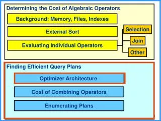
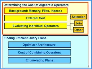
1. Determining the Cost of Algebraic Operators Background: Memory, Files, Indexes Selection External Sort Join Evaluating Individual Operators Other Finding Efficient Query Plans Optimizer Architecture Cost of Combining Operators Enumerating Plans

2. Types of Memory

3. The Memory Hierarchy • 3 types of memory: • main memory • disk • other: tapes, cds, dvds, etc. • We only discuss main memory and disk • others are mainly used for backup • Discussion takes a very simplified view of the memory, that is sufficient for our course

4. Main Memory • The main memory is randomly accessed • each piece of data can be returned in constant time, regardless of where it is located • Accessing the main memory is fast • And much faster than disk access • Main memory is expensive (relative to disk memory) • you have a few GB of main memory versus hundreds of GB of disk memory • Main memory is volatile • If computer shuts down, everything in main memory is lost

5. Tracks Arm movement Arm assembly Disk Spindle • Disk is: • Cheaper • Slower • Non-volatile • We will assume constant time to access values on disk (simplification, not true-to life) Disk head Sector Platters

6. Processing Data • In order to actually use data (e.g., read, perform computation, etc.) it must be in the main memory • Data on disk must be brought to the main memory for processing • Data is brought in units called blocks or pages • blocks have a set size • Whenever a tuple is needed the entire block which contains it must be brought!

7. Files • Files are simply sets of blocks • The blocks that make up a file may or may not be continuous in the disk memory • The part of the main memory used to read in blocks is called the buffer • An entire file may need to be read • It is possible that the entire file does not fit in the buffer • In this case as blocks are read, the buffer manager overwrites blocks that have already been brought

8. How it Works: Intuition Main Memory Buffer read R write S T Disk

9. Example(1) • Suppose that blocks are of size 1024 bytes • Suppose that a table has 100,000 tuples of 100 bytes each • No tuple is allowed to span two blocks • How many blocks are needed to store these tuples? • For each block 100*10 • Over all 100000/10 = 10000 blocks • How much space is “wasted”? • 10000*24 = 240000 bytes

10. Example (2) • Suppose that we want to compute the natural join of R and S • R spans N blocks • S spans M blocks • How can this be done if the buffer contains more than N+M blocks? • Load R and S to the buffer. • What problem is there if the buffer contains less than N+M blocks? (Solutions will be discussed later in the course)

11. What is Efficient? • Why do we have to even discuss the problem of evaluating relational algebra? • Can each operation be evaluated in polynomial time? yes • Can queries be evaluated in polynomial time? • No. the output can be exponential with the input size • New type of algorithms: External Algorithms

12. Measuring Complexity • Usually, the time to bring blocks from the disk to the main memory dominates the time needed to perform a computation • So, when analyzing runtime of algorithms to compute queries, we will always use the number of disk accessesas our complexity measure • Question: If the buffer contains more than N blocks, what is the complexity of sorting a table that takes up N blocks? • 2N (read the table + writ the table) • What if the buffer has less than N blocks

13. Types of Files

14. Tables are Stored in Files • Typically, all the tuples in a given table in the database are stored in files • The database takes over from the operating system all accesses to these files • Files can be organized in three different ways: • heap files • sorted files • indexed files

15. Types of Files • Heap file: • an unordered collection of tuples • tuples are inserted in arbitrary order (usually at the end, or first empty spot) • Sorted file: • tuples are sorted by some attribute (or set of attributes of the table) • Indexed file: • a data structure is present for quick access to tuples

16. Example • Consider a table S(A,B): • S has N tuples • K tuples fit in a block. • Answer each of the following if S is stored in a heap file • How long does it take to scan the entire S? • N/K (number of blocks S takes) = M • How long does it take to find all tuples with A=7? • M (go over the entire file) • How long does it take to insert a tuple into S? • 2 (read the last block to memory, add line and write to memory) • How long does it take to delete a tuple from S? • M+1 (M for finding the line + 1 for writing the corrected block)

17. Example • Consider a table S(A,B): • S has N tuples • K tuples fit in a block. • Answer each of the following if S is stored in a S is stored in a sorted file, based on A • How long does it take to scan the entire S? • M • How long does it take to find all tuples with A=7? • Log(M) + number of blocks with A=7 • How long does it take to insert a tuple into S? • Log(M) to find the right place + M/2 (avrg) blocks to read and write (fix) • How long does it take to delete a tuple from S? • Log(M) to find the place + M/2 (avrg) blocks to fix

18. Example • Consider a table S(A,B): • S has N tuples • K tuples fit in a block. • Answer each of the following if S is stored in a S is stored in a sorted file, based on B • How long does it take to scan the entire S? • M • How long does it take to find all tuples with A=7? • M • How long does it take to insert a tuple into S? • Log(M) + M/2 • How long does it take to delete a tuple from S? • Log(M) + M/2

19. In Practice • Maintenance of sorted files is so high, that they are generally not used • Instead, indexes are used to speed up the execution of the various operations • an index is a data structure that allows quick access to values based on a given key • Note the overloading of the word key:the key of the index is the attribute(s) used to search the index. It may or may not also be a key in the table

20. Indexes

21. Intuition: Index on Age 25 Efficiently Find Actual Data (on Disk): (Name, Age, Salary)

22. Intuition: Index on Age 25 36 43 47 36 Actual Data (on Disk): (Name, Age, Salary)

23. Index Organization • Rowid = Disk address for tuple: Address of block and number of tuple in block • Given a key k, the index can hold: • An actual tuple (with value k for key attribute) • A data entry <k,rowid>, (rowid for matching tuple) • A data entry <k,rowid-list>, (rowids for all matching tuples)

24. Different Alternatives • Alternative (1): An actual tuple (with value k for key attribute) • Then we say that the data is stored in an index-organized file • There can only be one index of this type for table • Can be used only when key attribute is primary key • We will normally assume Alternative (3)

25. Types of Indexes: Clustered/Unclustered • Clustered: When a file is organized such that the order of the tuples are similar to the order of data values in the index • Alternative (1) is clustered by definition • Alternative (3) is clustered if file is sorted on index key • Unclustered: Otherwise

26. Is the Index Clustered on Age? 25 36 43 47 36 Actual Data (on Disk): (Name, Age, Salary)

27. Is the Index Clustered on Salary? 9000 10000 15000 Actual Data (on Disk): (Name, Age, Salary)

28. Think About it • Why is clustering useful? • Which would be cheaper: finding all people of a certain age range, or all people with a specific salary range? • Can a table have clustered indexes on 2 different attributes? • E.g., clustered index for both age and salary?

29. Types of Indexes:Composite Keys • An index may be based on several attributes 43, 9000 43,10000 47,15000

30. Types of Indexes:Composite Keys • An index may be based on several attributes, e.g., age, sal age sal sal sal 43, 9000 43,10000 47,15000

31. Types of Indexes:Primary/Secondary • An index on a set of attributes that includes the primary key of the table is aprimary index. • Otherwise, the index is a secondary index • An index on a set of attributes that is unique is a uniqueindex • Questions: • Is a primary index a unique index? yes • Can a secondary index be a unique index? yes

32. Types of Indexes • The two most common types of indexes are B+ Tree indexes and Hash Indexes • Oracle also allows for bitmap indexes • We discuss B+ Tree indexes and Hash indexes briefly

33. Hash Tables

34. Hash Tables • A B+ Tree index can be used for equality queries and range queries. • A hash table index can be used only for equality queries.

35. What does it look like? • A hashtable is an array of pointers • Each pointer points to a linked list of pairs of "keys" and "values“ • By applying a hash function to a key, we can find its associated values, e.g., h(k) = mod(k,4) Key1, Value1 Key3, Value3 Key4, Value4 Hashtable of size 4 Key2, Value2

36. Are Hash tables Efficient? • How many disk accesses are needed to find workers who are 32 years old? 24, R35 28, R112 24, R76 32, R6 42, R111 Hashtable on Age 39, R52

37. Making Hash tables Efficient • Traditional hash tables have linked lists in which each node contains a single key-value pair • Instead, each node is chosen to be the size of a disk block • Has many key-value pairs • Usually length of hash table linked list will not be more than 3 blocks • Advantages? Disadvantages? • הרבה פחות קריאות לדיסק • בזבוז זכרון – בבלוק האחרון

38. B+ Trees

39. Before BTrees: Binary Search Trees • In a binary search tree, each node has a “key” • Values to the left of the key are smaller, values to the right are larger 6 3 7 1 4 2 5 How do we find the value 5?

40. 2 Other Binary Search Trees 1 4 7 2 6 6 5 7 1 3 5 4 3 How long does search take? 2

41. Problems with Binary Search Trees • Tree may be any length, so looking for a particular value may take a long time • When searching, each node has to be brought from disk to memory. This process is long, since nodes are small (i.e., many blocks must be read) • B+ Trees: • balanced • nodes are large

42. B+ Trees • B+ Trees are always balanced, i.e., the length of the path to every leaf is the same • B+ Trees keep similar-valued records together on a disk page, which takes advantage of locality of reference. • B+ Trees guarantee that every node in the tree will be full at least to a certain minimum percentage. This improves space efficiency while reducing the typical number of disk fetches necessary during a search or update operation.

43. Example B+ Tree • Search begins at root, and key comparisons direct it to a leaf • Search for 5*, 15*, all data entries >= 24* ... Root Many keys at each node 30 13 17 24 Tree is balanced 39* 3* 5* 19* 20* 22* 24* 27* 38* 2* 7* 14* 16* 29* 33* 34* • The list of rowids (missing in the picture)

44. Determining the Cost of Algebraic Operators Background: Memory, Files, Indexes Selection External Sort Join Evaluating Individual Operators Other Finding Efficient Query Plans Optimizer Architecture Cost of Combining Operators Enumerating Plans

45. Motivation • Sorted is needed for • ORDER BY clause • bulk loading into a BTree • duplicate elimination • some join algorithms • Problem: Data does not fit in main memory!!

46. Why You Should Understand How to Sort Large Sets of Items • Become a Google Employee • Become President of the USA • Eric Schmidt (CEO of Google): How do you determine good ways of sorting one million 32-bit integers in two megabytes of RAM? • Barack Obama: I think that bubble sort would be the wrong way to go

47. Think About it • Which sorting algorithm would you use? • Bubble sort? • Quick sort? (choose pivot, and then move values to the correct side of the pivot, recurse) • Merge sort? (recursively merge sorted subarrays) • We start by reviewing the standard merge sort algorithm, and then adapt for large data

48. MergeSort • A divide-and-conquer technique • Each unsorted collection is split into 2 • Then again • Then again • Then again • ……. Until we have collections of size 1 • Now we merge sorted collections • Then again • Then again • Then again • Until we merge the two halves

49. MergeSort(array a, indexes low, high) • If (low < high) • middle(low + high)/2 • MergeSort(a,low,middle) // split 1 • MergeSort(a,middle+1,high) // split 2 • Merge(a,low,middle,high) // merge 1+2

50. Merge(arrays a, index low, mid, high) bempty array, pHmid+1, ilow, pLlow while (pL<=mid AND pH<=high) if (a[pL]<=a[pH]) b[i]a[pL] ii+1, pLpL+1 else b[i]a[pH] ii+1, pHpH+1 if pL<=mid copy a[pL…mid] into b[i…] elseif pH<=high copy a[pH…high] into b[i…] copy b[low…high] onto a[low…high]