Download
1 / 23
230 likes | 413 Vues
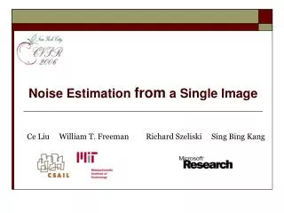
Accepted for publication by IEEE Transactions on Pattern Analysis and Machine Intelligence. Automatic Estimation and Removal of Noise from a Single Image. Ce Liu * Richard Szeliski † Sing Bing Kang † C. Lawrence Zitnick † William T. Freeman * * CSAIL, MIT

E N D
Accepted for publication by IEEE Transactions on Pattern Analysis and Machine Intelligence Automatic Estimation and Removal of Noise from a Single Image Ce Liu* Richard Szeliski† Sing Bing Kang† C. Lawrence Zitnick† William T. Freeman* *CSAIL, MIT †Microsoft Research
The criteria of image denoising • Perceptually flat regions should be flat • Image boundaries should be preserved (neither blurred or sharpened) • Texture details should not be lost • Global contrast should be preserved • No artifacts should be generated
Denoising is hard… • Different source and type of noise • How strong is the noise? • Locally, it is hard to distinguish • Texture vs. noise • Object boundary vs. structural noise • Speed? Quality?
Related work • Wavelets (coring, GSM) • Anisotropic diffusion (PDEs) • FRAME & FOE • Bilateral filtering • Nonlocal methods • Conditional Random Fields
Segmentation-based piecewise smooth image models • An image can be reconstructed by • Over-segmentation (your favorite method) • Affine reconstruction for each segment (RGB is an affine function of xy) • Boundary blur estimation Piecewise smooth image reconstruction
Piecewise smooth reconstruction (a) Original image (b) Segmentation (c) Per-segment affine reconstruction (d) Affine reconstruction + boundary blur
Important properties of piecewise smooth image model • Piecewise smooth image model is consistent with sparse image prior horizontal vertical Filter responses Piecewise smooth reconstruction
Important properties of piecewise smooth image model • The color distribution per segment can be well approximated by a line segment Sorted eigenvalues in RGB space for each segment. The reddish picture indicates that the largest eigenvalue is significantly bigger than the second and third RGB values projected onto the eigenvector w.r.t. the largest eigenvalue. It is almost identical to the original image.
s s s Residual std. dev. I I I Brightness Important properties of piecewise smooth image model • The standard deviation of residual per each segment is the upper bound of the noise level in that segment • Assume brightness mean I is accurate estimate • Standard deviation s is an over-estimate: (may contain signal) • The lower envelope is the upper bound of noise level function (NLF)
Segmentation-based noise reduction • The noise level (std dev) for each segment, each RGB channel (from the inferred NLF) • 0th-order model • Assume the pixel is independent of the neighbors (of course this is not true) • Bayesian MAP inference for each pixel (trivial)
1st order Gaussian CRF • Of course the neighboring pixels are dependent • A Gaussian conditional random field (GCRF) is formed to incorporate • Distance to noise • Distance to signal • Image-dependent regularization • Inference by conjugate gradient method
Experimental results • 17 images are randomly selected from Berkeley image segmentation database • Compare to bilateral filtering, curvature preserving PDE and wavelet GSM.
Visual inspection 10% AWGN PDE Wavelet GSM Ours Original
Close-up view 10% AWGN PDE Wavelet GSM Ours Original
Visual inspection 10% AWGN PDE Wavelet GSM Ours Original
Close-up view 10% AWGN PDE Wavelet GSM Ours Original
Apply to real CCD noise Estimated NLF
Close-up view Since wavelet GSM only takes one constant noise level, it either over-smoothes (as s =15%) or under-smoothes (s =10%). We estimate signal-dependent noise level (NLF), and our approach handles both high and low noise level well. Estimated NLF
A very challenging example Real digital camera noise (low light, high ISO) Denoised by wavelet GSM Denoised by our model Estimated NLF
Conclusion • Noise estimation and removal using one framework: piecewise smooth image model • The chrominance component of the noise can be significantly reduced by simple projection • Computer vision algorithms can be automated by estimating the peripheral parameters such as noise level, blur level, lighting, …