Download
1 / 86
920 likes | 1.37k Vues
Part 3 PRODUCTION AND SUPPLY PRODUCTION FUNCTIONS COST FUNCTION PROFIT MAXINIZATION. Chapter 7. PRODUCTION FUNCTIONS. Contents. Marginal productivity Isoquant Maps and the rate of technical substitution Returns to Scale The elasticity of substitution Four simple production function

E N D
Part 3 PRODUCTION AND SUPPLY • PRODUCTION FUNCTIONS • COST FUNCTION • PROFIT MAXINIZATION
Chapter 7 PRODUCTION FUNCTIONS
Contents • Marginal productivity • Isoquant Maps and the rate of technical substitution • Returns to Scale • The elasticity of substitution • Four simple production function • Technical progress
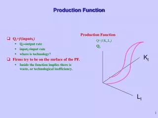
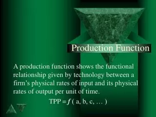
Production Function • The firm’s production function for a particular good (q) shows the maximum amount of the good that can be produced using alternative combinations of capital (k) and labor (l) q = f(k,l)
Average Physical Product • Labor productivity is often measured by average productivity • Note that APl also depends on the amount of capital employed
Marginal Physical Product • To study variation in a single input, we define marginal physical product as the additional output that can be produced by employing one more unit of that input while holding other inputs constant
Diminishing Marginal Productivity • The marginal physical product of an input depends on how much of that input is used • In general, we assume diminishing marginal productivity
Diminishing Marginal Productivity • Because of diminishing marginal productivity, 19th century economist Thomas Malthus worried about the effect of population growth on labor productivity • But changes in the marginal productivity of labor over time also depend on changes in other inputs such as capital • we need to consider flk which is often > 0
Isoquant Maps • To illustrate the possible substitution of one input for another, we use an isoquant map • An isoquant shows those combinations of k and l that can produce a given level of output (q0) f(k,l) = q0
Each isoquant represents a different level of output • output rises as we move northeast q = 30 q = 20 Isoquant Map k per period l per period
Isoquant Maps Production Function : Multiple Inputs
The slope of an isoquant shows the rate at which l can be substituted for k A kA B kB lA lB Marginal Rate of Technical Substitution (RTS) k per period - slope = marginal rate of technical substitution (RTS) RTS > 0 and is diminishing for increasing inputs of labor q = 20 l per period
Marginal Rate of Technical Substitution (RTS) • The marginal rate of technical substitution (RTS) shows the rate at which labor can be substituted for capital while holding output constant along an isoquant
RTS and Marginal Productivities • Take the total differential of the production function: • Along an isoquant dq = 0, so
RTS and Marginal Productivities • Because MPl and MPk will both be nonnegative, RTS will be positive (or zero) • However, it is generally not possible to derive a diminishing RTSfrom the assumption of diminishing marginal productivity alone
RTS and Marginal Productivities • To show that isoquants are convex, we would like to show that d(RTS)/dl < 0 • Since RTS = fl/fk
RTS and Marginal Productivities • Using the fact that dk/dl = -fl/fk along an isoquant and Young’s theorem (fkl = flk) • Because we have assumed fk > 0, the denominator is positive • Because fll and fkk are both assumed to be negative, the ratio will be negative if fkl is positive quasi-concave function
RTS and Marginal Productivities • Intuitively, it seems reasonable that fkl= flk should be positive • if workers have more capital, they will be more productive • But some production functions have fkl < 0 over some input ranges • when we assume diminishing RTS we are assuming that MPl and MPk diminish quickly enough to compensate for any possible negative cross-productivity effects
If the production function is given by q = f(k,l) and all inputs are multiplied by the same positive constant (t >1), then Returns to Scale
Returns to Scale • It is possible for a production function to exhibit constant returns to scale for some levels of input usage and increasing or decreasing returns for other levels • economists refer to the degree of returns to scale with the implicit notion that only a fairly narrow range of variation in input usage and the related level of output is being considered
Constant Returns to Scale Labor(hours)
Constant Returns to Scale • Constant returns-to-scale production functions are homogeneous of degree one in inputs f(tk,tl) = t1f(k,l) = tq • This implies that the marginal productivity functions are homogeneous of degree zero • if a function is homogeneous of degree k, its derivatives are homogeneous of degree k-1
Constant Returns to Scale • The marginal productivity of any input depends on the ratio of capital and labor (not on the absolute levels of these inputs) • The RTS between k and l depends only on the ratio of k to l, not the scale of operation
The isoquants are equally spaced as output expands q = 3 q = 2 q = 1 Constant Returns to Scale • The production function will be homothetic • Geometrically, all of the isoquants are radial expansions of one another • Along a ray from the origin (constant k/l), the RTS will be the same on all isoquants k per period l per period
homothetic production function • The IRS and DRS also have a homothetic difference indifference curve , because the property of homotheticity is retained by any monotonic transformation of homogeneous function