Production Function, Factor Market and Aggregate Supply Function
Production Function, Factor Market and Aggregate Supply Function. CHAPTER 9. 1. Determinants of Output and Price. Chapter 9. * Output (real income), employment and price / inflation are determined by. Aggregate supply (AS) and Aggregate demand (AD) * Each of which is governed by


Production Function, Factor Market and Aggregate Supply Function
E N D
Presentation Transcript
Production Function, Factor Market and Aggregate Supply Function CHAPTER 9
1. Determinants of Output and Price Chapter 9 * Output (real income), employment and price / inflation are determined by • Aggregate supply (AS) and • Aggregate demand (AD) * Each of which is governed by • Market and government rules * What areAS and AD ? • AS depicts supply of all goods & services at various (minimum) prices • AD gives demand for all goods & services at various (maximum) prices
2. Aggregate Supply Curve Vs. Industry Supply Curve • Aggregate supply (AS) is more flexible than industry supply (IS) in the short-run and vice versa in the long-run, because - Resources (factors of production) could be employed over time (extra shift) for some time but not for all the time - Resources of an economy are fixed but those of an industry are flexible in the long-run Accordingly, • AS curve is flatter than IS in the short-run • AS curve is steeper than IS curve in long-run
3. Aggregate Supply • * Aggregate supply depends on two forces: • Potential output, which is governed by - Quantities and qualities of inputs, including technology (production function) [ full employment ] • Actual output, which is influenced additionally by - Inputs’ employment, which, in turn is affected by - inputs’ & product prices (shut down price)
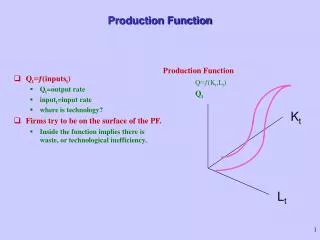
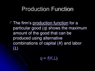
5. Production Function Y = f ( L , K ,T ) (9.1) f1 , f2 , f3 > 0 Figure 9.1: Prod Function • Law of diminishing m. return (non-linear prod. function) • MPP of a factor varies directly with quantity of other factors. Thus, labour productivity is higher in USA than India.
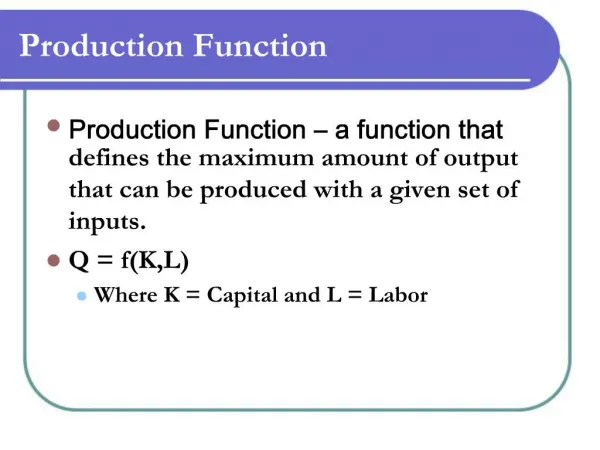
6. Demand for FOP (Labour and Capital) • Firms’ optimum behavior • Perfect competition in the product market Q = f (L, K) (9.2) C = L W + K R (9.3) Profit = TR – TC = f (L, K) P - L W – K R • Optimisation would give MRP of labour = Marginal cost of labour MRP of capital = Marginal cost of capital
6. Demand for FOP- contd. * Under perfect condition, in both product and factor market, the above conditions reduce to MPP of labour = (9.4) MPP of capital = (9.5) • Interdependence of production and factor demand functions DL : MPPL = W / P & DK : MPPK = R / P The 2nd order condition of optimization would limit the above conditions to the rising part of the corresponding MPPs.
6. Demand for FOP – contd. Example: * Cobb-Douglas (constant returns) function Q = A La K1-a (9.6) * Optimisationyields [(1-a) (Q/L)] / [a (Q/K)] = W / R * Labour demand L = [(1-a)/a]a [ R/W]a [ Q/A] (9.7) * Capital demand K = [a/(1-a)]1-a [W/R]1-a [Q/A] (9.8)
7. Labour Supply Function • Worker’s optimum behaviour * Income - Leisure trade-off Maximize U = f(Y, F) f1, f2 > 0 Subject to Y = (T - F)(W / P) (Where, Y = real income, T = total time F = leisure / free time) * Optimization gives MRSY, F = fF / fY = W / P (9.11) Or, SL function : MRSY, F = W / P The above assumes no market frictions, like trade union, cartel or govt. regulations on wage, retirement age, etc.
7. Labour Supply Function – contd. • Backward bending labour supply curve • Income and substitution effects of a • change in wage rate on SL • - Substitution effect is always positive • - Income effect is ambiguous, positive at low income and negative at high income • Shifters of SL curve Supply of labour curve shifts with changes in non - wage determinants of labour supply, which follow.
7. Labour Supply Function – contd. • Labour supply curve shifts down (= SL increases) when there is a. Increase in population b. Increase in work force participation rate c. Increase in working hours/day • d. liberalisation in immigration policy e. Increase in minimum wage f. Increase in retirement age g. Decrease in unemployment benefits • Increase in preference for work relative to leisure • Increase in over time wage vis-à-vis regular wage rate • j. And so on • And vice versa • => Supply side economics ingredients
8. Capital Supply Function • Capital renters optimizing behaviour • Upward sloping • Shifts down (SK increases) if there is • a.Increase in propensity to save / invest b.Increase in the risk - preference of firms c. Increase in tax incentives for investments d. Liberalisation of foreign investments e. Improvements in property rights f. And so on => Supply side economics ingredients
9. Factor Market Equilibrium- Labour Real Wage SL W Po DL O Figure 9.4: Labour market equilibrium : Flex wage (Classical) Quantity of labour => Full Employment
10. Factor Market Equilibrium: Capital Real Wage W0 P2 Wo Po W0 P1 DL 0 L2 Lo L1 Labour Figure 9.5 : Labour Market under Fixed Nominal Wage Rate (Keynesian): W0 • Workers supply as much labour as firms demand at W0. • Firms DL varies inversely with price
11. AS Curve under Wage-Price Flexibility W Price I 1 W 0 W II 2 AS P 1 P 0 P 2 Real Wage (W/P) Y Output 0 0 F SL LF IV III Y Labour DL Figure 9.6: AS curve under wage-price flexibility: Classical assumption (no friction) ,
11. AS Curve under Wage-Price Flexibility- contd. • Implications • AS curve vertical at YF (Full employment equilibrium) • Output is totally supply determined (Say’s law) • Price and nominal wage are directly and proportionally related (W / P = constant) • Price is demand determined
12. AS curve under Price Rigidity (Flex Money / Real wage) • Why fixed price? - Menu cost - Price contracts / brochures - Staggered price contracts - Competition on price front • Wage bargains in terms of money wage • Firms supply any output at the fixed price • => firms ignore their labor demand curve
12. AS curve under Price Rigidity- contd. Figure 9.7: As Curve under Price Rigidity
12. AS curve under Price Rigidity – contd. • Implications • AS curve is inverted L – shaped • Output is demand determined • Price is fixed by contract between buyers / sellers • - Brochures • Mark up moves counter - cyclically • Nominal and real wage rates move pro - cyclical
13. AS Curve under Nominal Wage Rigidity (Flexible Price) • Why nominal wage rigidity ? - Workers interested both in absolute and relative wage - Minimum wage regulation - Monopoly power of unions - Efficiency wage theory / Insider-outsider theory • Wage contracts - Formal / informal - In money wage, not always indexed => Workers supply any labour at the fixed wage
13. AS curve under Nominal Wage Rigidity – contd. Price AS I W 0 II B P 1 P0 A C P 2 D P 3 0 Y Y Y W W W W Real Wage Output 0 0 0 0 3 2 F P P P P 2 0 3 1 L 3 L 2 L F L 1 III Labour IV Figure 9.8: AS curve under Nominal Wage Rigidity
13. AS curve under Nominal Wage Rigidity – contd. • Implications • - Labour employment is determined solely by DL • - AS curve slopes upward • - Real wage movements are counter cyclical • - Workers suffer from money illusion
13. AS curve under Nominal Wage Rigidity – contd. • Applications • U.K. data suggest that during 1929 - 36, • - Unemployment rate was high • - Money wage rate fell by 5% only initially, and even rose subsequently • - Even real wage rate did not fall to clear unemployment • => Nominal wage rigidity is a feasible assumption in the short-run
14. AS curve Flexible Money Wage / Price: Some Prices Fixed, others variable • General price = weighted average of many prices. • In short-run, some prices (P1) may be fixed while some other (P2) flexible. Under such a situation (i) P1 = Pe (ii) P2 = P + a (Y – Yn) P = λ Pe + (1 - λ) [ P + a ( Y – Yn ) ] (where λ is the fraction of firms having sticky prices) Solution of the above equation would give Y = Yn + α ( P – Pe ) (9.9) (where α = λ / a (1 - λ) ≤ 1) Equation (9.9) gives the upward sloping AS curve.
15. AS curve under Flexible Money Wage / Price: Friedman - Lucas Mistaken Expectations • Friedman’s Asymmetric Information / Worker’s Fooling Model: • DL = f (W / P) and SL = f (W / Pe) • * AD↑ => Pˆ • firms know this but • workers do not • => DLˆ => ASˆ * Thus, as price goes up. AS goes up and vice versa => AS curve slopes upward !
15. AS curve under Flexible Money Wage / Price: Friedman - Lucas Mistaken Expectations- contd. • Lucas’s Information Barrier • * ADˆ => Pˆ • * Neither firms nor workers know this • * Each firm thinks the • - price of its own product alone (relative • price) is up • => DLˆ and there by ASˆ Thus, as price is up, AS is up => * AS curve slopes upward * W/P is counter cyclical, and * W/Pe is pro cyclical
C Price . P0 B A . O YF Output 16. Short and Long Run AS curves Figure 9.9: Short / Long - Run AS curves a. P0BC is the short - run AS curve under price rigidity b. ABC is the short - run AS curve under nominal wage rigidity / Flexible nominal wage but some fixed some flex prices / fooling of workers / information barrier c. YFBC is the long - run AS curve under full wage - price flexibility and perfect information. Crucial difference: Price fixed in short run, flexible in long run
17. Shifts in AS Curve: Supply Shocks • Shifts in AS could be caused by changes in • labour force • capital (structures, business equipment • and inventories) • c. materials and supplies • energy resources / oil price • inputs’ prices • and the level of • f. technology (factor productivity)/ industrial peace • g. weather conditions/environment/natural factors • and, as we shall see later, • h. expected inflation
18. AS Function / Equation * Friedman - Lucas Version * Expected Price Augmented AS Function (9.9) > 0 * Slopes upward • * Slope equals • - larger the % of fixed prices, the flatter is AS curve • Position depends on Yn , Pe and • Short - run function is given by (9.9) • In long-run, P = Pe and thus, • Y = Yn (9.10)
19. Phillips’ Curve Equation • * Money Wage function: • W = f (ADL – ASL) • f1 > 0 • where, • ADL = Labour employed + Vacancies • ASL = Labour employed + Unemployment • ADL – ASL = Vacancies - Unemployment = - U (in the absence of data on vacancies => Money wage and unemployment rate are negatively related
19. Phillips’ Curve Equation – contd. • US estimates: 1950 - 66 data: w = - 1.43 + 8.27 (1/u) R2 = 0.38 • * Function is non – linear in w and u • * In w and u axes, it slopes down ward • * For w = 0, u = 5.8; and for w = 2, u = 2.4 • * At w = - 1.43, u = infinity • * It is convex to the origin
19. Phillips’ Curve Equation – contd. . = - b - W ( u u ) (9.11) n • Incorporating natural rate of unemployment: • Un = NAIRU = LSUR • Three components of Un : • - Frictional U • - Structural U • - Seasonal
19. Phillips’ Curve Equation – contd. = - b - P ( u u ) . n - Permanent trade-off between P and u . . = - b - e P P ( u u ) (9.13) n . (9.14) = - b - + n e P P ( u u ) n • Samuelson - Solow modification: . (9.12) • Inflation - Augmented • Supply Shocks incorporated * Short (SP) and long-run Phillips curve (LP) * LP: Correct expectations line * Temporary trade-off only * Over - heated economy
19. Phillips’ Curve Equation – contd. . P 2 . . ( ) e P P SP = . 2 2 P 1 . . u u ) ( e P P SP b n = . 2 1 P . . ( 0 ) e P P SP = 0 0 LP Inflation Rate D E B C A O Unemployment Rate Figure 9. 10: Phillips Curves
19. Phillips’ Curve Equation – contd. • Position of Phillips curve depends * Positively and one to one on - expected inflation rate, and - adverse supply shock * Positively on natural rate of unemployment • Negatively on deviation of unemployment rate from its natural rate (= u-un = cyclical rate of unemployment) • Slope of Phillips curve is negative and its magnitude depends on the • * Sensitiveness of inflation rate to the deviation of u from un
20. Phillips’ Curve vis a vis AS Function • Phillips curve and AS function are closely • related: - Rewriting Phillips’ curve: - Subtraction of the lagged P gives
20. Phillips’ Curve vis a vis AS Function – contd. . 1 e = + - P P ( Y Y ) n a * Treating the variables as logs gives * Recall Okun’s law ( Y-Yn ) = f ( u - un ) f1 < 0 Or, Note: USA: % change in real GDP = 3% - 2 [change in unemployment rate] • Substitution of this Okun’s equation into above Phillips • curve gives
20. Phillips’ Curve vis -a- vis AS Function – contd. e = - b - P P ( u u ) n 1 e = + - + n P P ( Y Y ) n a . . * Substitution from the Okun’s law and inclusion of supply shock gives . . (9.15) • => Same as AS function (9.9) • Trade off between growth and price stability • M Friedman used Un concept to show limitation of monetary policy for not being able to reduce u below Un without endangering inflation
21. Adaptive Expectations’ Model • Sluggishness / inertial in the economy • Backward looking theory = w1Pt + w2Pt-1+ w3Pt-2 + .... = a Pt + a(1-a) Pt-1 + a(1-a)2 Pt-2 + .... (9.16) S = a + a(1-1) + a(1-a)2 + ..... = 1 = = a Pt-1 + a(1-a) Pt-2 + a(1-a)2 Pt-3 + ....
21. Adaptive Expectations’ Model – contd. By subtracting the latter from the former, Or, (9.17) • Limitations • Prone to Systematic errors • Ignore all other (non-own past values) • factors
22. Rational Expectations Hypothesis • Forward looking theory • Full information theory • Expectations based on • Current price • Past prices • Current and past values of all the variables which impinge on the price • Expected / systematic policy actions and non-policy events which have bearings on the future price. • Smart use of the above information • no formula but rational behaviour • May not give right forecasts but no systematic error
22. Rational Expectations Hypothesis – contd. • Limitations • No formula and thus some what subjective • Prohibitive Information cost • Worth of the additional information uncertain • Imperfect information • Policy surprises
23. Conclusion • Allows price flexibility • Recognises resource constraint • Keynes had ignored price expectations • Little consensus on AS curve • Short run and long run AS curves, distinguished on the basis of wage-price rigidity and flexibility, respectively • AS curve is vertical at Yn in the long run - upward sloping in short (medium) run, and - horizontal at fixed P in the very short run • AS curve slopes upward basically due to - law of diminishing marginal returns, and - increasing pressure on money wage to rise as output and employment increase