Download
1 / 34
340 likes | 354 Vues
This presentation by James Reeler explores the evidence of anthropogenic climate change, including climate variation, climate change, and sources of data such as instrumental measurements and proxy data.

E N D
Introduction: the evidence for anthropogenic climate change Presented by James Reeler UWC
Climate variation • All manner of human and natural activities are affected by weather and climate • WEATHER is the day to day effect of natural conditions. • CLIMATE refers to an averaging of these conditions over a longer period, obtaining a general picture of trends in conditions over time. • Both systems are highly variable. • Climate is influenced on varying time scales by factors such as fluctuations in solar output, the Earth’s orbit, changes in vegetation cover and in the gaseous composition of the atmosphere (IPCC, 2001). • This short-term variation is termed climate variability, or CLIMATE VARIATION.
Climate change • A long term trend in climatic conditions away from the established conditions is termed CLIMATE CHANGE. • The earth has always experienced climate change due to natural variations in insolation and atmospheric conditions– it is not a new process. • Orogeny, which is the development of new surface features on a geological time scale, can affect the climate gradually. • The most recent ice age ended 10 000 years ago, and what we have been experiencing in recent history may be termed a “climatic optimum” • It is telling that agriculture only arose as a human adaptation strategy within the last few thousand years, corresponding to optimal growth conditions for agricultural crops. Source: Canadian Institute for Climate Studies
Source: IPCC online talks What are we looking for? • Changing climatic variables could be expressed in different ways, depending on how the climate is transformed. • A change in mean temperature would mean we would see more extreme heat and hot weather events. • A transformation in variance of temperature would give a broader spread, resulting in more extremes of both heat and cold. • If there were a change in both mean and variance of temperature, whilst we would see more extreme heat and warm weather, we might still observe extremes of cold weather. • This type of change might therefore hide the signal, since certain areas would be unchanged. Only after extensive observation would the trend be clear. This may be what has happened in recent history
Sources of data - instrumental • Instrumental measurement of climate variables is an important data source, although we only have true records for a short historical period. • Using standard instruments, we record: • Temperature • Rainfall • Wind • Humidity • Atmospheric aerosol and gas concentrations • These standard variables allow measurement of change in the earth’s systems.
Temperature • Temperature is an essential indicator variable, because it provides us with a direct measurement of the energy in the earth’s atmospheric system. • Temperature records date from the middle of the 19th century. • Surface air temperature is usually measured at weather stations by means of mercury or alcohol thermometers. • However, much recent work has been done to allow measurement of the temperature of other atmospheric levels, using the TIROS-N series of satellites. • These atmospheric temperature records start in 1958 (conventional radiosonde network)(Angell, 1988) and 1979 (microwave-sounding unit) (Spencer & Christy, 1990) respectively.
Palaeoclimate reconstruction from proxy data • In order to obtain data prior to the advent of modern measuring devices, climatologists resort to using proxy data from a variety of sources. • Sources of proxy data include: • Glaciological (ice cores) • Oxygen isotopes • Trace elements and microparticle concentrations • Physical properties • Geological • Sediments • Marine – organic/inorganic sediments • Terrestrial – glacial / periglacial/ aeolian/ lacustrine • Sedimentary rocks • Facies analysis • Fossil/microfossil analysis • Mineral analysis • Isotope geochemistry • Biological • Tree rings (dendroclimatology) • Pollen species/abundances • Insects • Historical • Historical meteorological records • Parameteorological records (environmental indicators) • Phenological records (biological indicators)
Palaeoclimatological time scale ProxyTime period before present (years) 10910810710610510410310210 Historical Tree rings, pollen Ice cores Glacial deposits Marine organic sediments Inorganic sediments Sedimentary rocks Decreasing resolution (and accuracy)
Proxy data sources: Ice cores • Data from ice cores is extracted in a number of ways. • Oxygen isotopic analysis gives an idea of the temperature at which the ice was deposited (since O18 has a higher vapour pressure, it is preferentially deposited).. In warmer conditions, more O18 will be found in the polar ice (Craig, 1961 ; Morgan, 1982). • Atmospheric gas concentrations can be extracted from bubbles formed by the closing off of air pores as firn turns to ice. (Raynaud & Lorius, 1973) . • Physical variations in ice structure such as crystal size, incidence of melts and number/structure of bubbles give an idea of temperature and frequency of melt periods or deposition (Langway, 1970; Koerner, 1977).
Proxy data sources: Dendroclimatology • The pattern of growth of trees is laid down within their structure, providing a high-resolution (annual) picture of climatic variables in the Holocene. • Much can be deduced from growth bands – the thickness corresponds to the favourability of climatic conditions (light, temperature, rainfall, windspeed) (Bradley,1985; Fritts, 1976). • The density of the bands says much about the growing season (latewood is much denser than earlywood) (Schweingruber et al., 1978). • Isotopic analysis of the bands can also give us information about the climatic conditions. (Epstein et al., 1976). • By studying a number of trees in an area of a similar age, a statistically sound analysis of conditions can be obtained.
Proxy data sources: Oceanic sediments • Preferential uptake of O18 under cool conditions by fossilized plankton allows analysis of the temperature of deposition by isotopic analysis. (Urey, 1948). • Species assemblages show variation in the number of warm- and cold-water plankton species. (Williams & Johnson, 1975) • Morphological variations are expressed by a number of species in response to climatic variables. (Kennett,1976). • The content of terrigeneous material in sediments corresponds to continental weathering. Consequently, the purity of the calcareous ooze gives a strong indication of the extent of weathering. (Hays & Perruzza,1972). • The chemical and physical processes affecting the inorganic sediments prior to deposition correspond to particular climate regimes. (Kolla et al., 1979).
Proxy data sources: Other • Glacial moraines give a rough picture of glacial advances and retreats, but successive movements which erase each other, as well as difficulties in dating moraines, limit the application. • Lacustrine (lake) size variation, especially in arid areas, can be significant, so stratigraphic and microfossil analysis can give some indication of climate variation. • Pollen accumulates on all surfaces, and is useful for palaeoclimatic deduction. However, the many difficulties associated with analysis mean that only qualititative comparisons are feasible. • Sedimentary rocks can provide data through facies analysis (rock types), assessment of fossils and microfossils, and analysis of sediment grain size/rate of deposition. However, the resolution of these data is very low (thousands of years).
The role of climate models • Once historical and palaeoclimatological data have been gathered, we have some idea of: • How the climate has changed in the past • What atmospheric and biological conditions were associated with this change • This allows us to build and test models of the interaction of climatic variables • These models allow us some capacity to then establish how a given change in certain factors will affect future climate. • This becomes the basis for assessment of the current state of the environment • We will go into this in more detail in chapter 2.
Evidence for change • So, what evidence is there for anthropogenic change? • By comparing current data and measurements with historical and palaeclimatological data, we have obtained a good picture of the climate over the last several thousand years. • It is clear that there has been a significant transformation of the climate over the last hundred years, and that the rate of change is increasing. • Signal analysis and modelling has proved that this change cannot be attributed to processes other than human interaction with the environment.
Decrease in cumulative net balance over the period 1975- 2003 Source: World Glacier Monitoring Service Thermal indicators: Glacial melting • The change in size of glaciers is measured by their mass balance: the net annual gain/loss of mass at the glacier surface per unit surface area. • This is useful because it measures the contribution of glacial melt to sea level rise. • Almost all glaciers have been shown to be retreating. (IAHS (ICSI)/UNEP/UNESCO, 1998) • Some glaciers in Norway and New Zealand are advancing, but this is because of increased precipitation due to warmer weather. • Exposure of radiocarbon-dated ancient remains in high saddles in the Alps shows recession is reaching levels not seen for thousands of years • This ice has not melted for thousands of years, hence the finding of the 5000 year-old Oetzal “ice man”. (IPCC, 2004) Glacial retreat over a 98-year period in Glacier National Park , USA. Glacier National ParkArchives/F.E. Mathes (1900), USGS/L. McKeon (1998)
Thermal indicators: Sea ice • Comprehensive Antarctic sea ice records date from the 1970s, although there is considerable data prior to this point for the Arctic. (Parkinson, 2000). • A considerable decrease in sea ice thickness over the 1978-1996 period has been observed (Parkinson et al., 1999). • Satellite data has shown a considerable decrease in the extent of sea ice. • This is particularly evident in the collapse of the Larsen B ice shelf in 2002. • Four other major ice shelves have retreated (Vaughan and Doake, 1996). • Sea ice melt does not contribute to sea-level rise, since it is already in the ocean.
Thermal indicators: permafrost • About 25% of the Northern Hemisphere landmass is under permafrost , including much of Canada, China, Russia and Alaska (Brown et al., 1997). • Significant portions of this area are now undergoing melting as a result of raised temperatures. • This is seen through the sudden appearance of potholes of considerable size and the draining of many lakes as their frozen base is removed. • However, direct measurement of the melting of permafrost has been gathered over the last twenty years in many regions of the world (Gravis et al., 1988; Weller and Anderson, 1998; Romanovsky and Osterkamp, 1999) • Onset, magnitude and extent of permafrost melting varies from area to area. A pothole formed by melting permafrost. You can see still frozen ice at the back of the hole. Source: Romanovsky, Fairbanks Alaska.
Thermal indicators: Sea level change • Sea level has risen by an average of 15 cm over the last century (IPCC 2001). • Melting of sea ice does not increase the level of the oceans. • However, as the ice Antarctic ice sheet retreats, it is increasing polar glaciers’ access to the ocean. • As their flow increases under SOURCE: IPCC website gravity, they will likely contribute more to the rise in sea level. The extent and rate of this influx is a subject of much research. • In addition to the increasing amount of water flowing into the oceans, the sea level is likely to rise due to thermal expansion. Simulations predict that ultimate levels could reach as much as . an additional 2m at equilibrium.
Source: UK Meterological Office Source: IPCC Thermal indicators: Sea temperatures • Sea temperatures have been gradually increasing worldwide. • Measurements in the 19th century were somewhat inaccurate, but this is taken into account through a correction factor. • Immediate effects of this will include a change in the capacity of seawater to absorb CO2. • Long term concerns of such a trend include the shutting down or movement of oceanic currents such as the “conveyor belt”, ironically reducing air temperature in areas of atmospheric heat release . • More importantly, the deep saline currents provide many nutrients for surface ecosystems fed by plankton. A reduction in oceanic plankton will limit another important carbon sink, since many species have carbonate shells. It may also cause a crash in oceanic biodiversity.
Source: IPCC Third Assessment Report Is oceanic circulation changing? • The El Niño Southern Oscillation is a current system that is the primary global mode of variation on the 2 to 7 year time interval, typified by a change in SST anomaly. (IPCC, 2001). • ENSO is associated with extreme climatic events . • Multiproxy reconstruction of ENSO suggests recent extremes are outside the norms of historic conditions. • The 1990s in particular show trends outside the norms of previous decades, including reduced variability (more El Niño events with reduced occurrence of the corollary cool La Niña) (Goddard and Graham, 1997). • Similar statistical anomalies have been observed in both the North Atlantic Oscillation and the North Pacific Oscillation. • These anomalies may be part of a larger variation, or may be part of the natural cycle – it is too early to determine for certain at this stage.
The greenhouse effect • To some extent, life on earth is contingent on the greenhouse effect – without it the earth’s surface temperature would be considerably below the freezing point of water. • Certain gases are opaque at infra-red light frequencies. These include methane, water vapour, nitrous oxides, ozone, and most importantly, CO2. Source: ARIC • Some short wave solar radiation is converted to long wave infra red at the earth’s surface. This is then absorbed by greenhouse gases, raising the atmospheric temperature. • As the proportion of greenhouse gases in the atmosphere increases, so does the potential for absorption of radiation, effectively raising the temperature. • This effect, and the dangers of increased carbon dioxide emissions wasoutlined by Svante Arrhenius over a century ago! (Arrhenius, 1896).
Climate change forcings • The effect of various factors on the climate are expressed as a forcing value (ie: to what extent they force global warming) • The forcing value is measured in Wm-2 (the increase in effective energy caused per square metre). • Forcings are discussed in more detail in the next chapter, on GCMs, but for now it is important to understand that there are many sources of climate forcing. • However, human activity has introduced significant radiative forcing to the atmosphere through various factors, and these will be touched upon in the next couple of slides. Source: Mauna Loa Observatory
Source: IPCC Third Assessment Report Greenhouse gases: methane • Since the beginning of the industrial revolution, and most particularly in the last century with the widespread use of the internal combustion engine, atmospheric concentrations of greenhouse gases have climbed massively. • Methane (CH4), is produced by domestic animals in large quantities. • Also produced by all anaerobic decomposition (notably in landfills, hydroelectric dams and rice paddies). (Prather et al.,1995). • Forcing increase relative to 1765 (Wm-2): • 19001960197019801990 • 0.10.240.300.360.42
Source: IPCC Third Assessment Report Greenhouse gases: nitrous oxide • Nitrous oxide (N2O) is naturally produced by biological functions in the soil and oceans. • Anthropogenic sources include industrial combustion, vehicle exhausts, biomass burning and the use of chemical fertilisers. • Forcing increase relative to 1765 (Wm-2): • 19001960197019801990 • 0.0270.0450.0540.0680.10
Carbon dioxide is emitted by all combustion, particularly fossil fuels used for engine fuels and energy generation. Burning of forests also emits CO2, as well as reducing their capacity for carbon sequestration. Greenhouse gases: carbon dioxide Source: IPCC Third Assessment Report • At this stage CO2 is the largest anthropogenic contribution to climatic forcing. Levels are higher than at any time in the past 450 000 years. • Forcing increase relative to 1765 (Wm-2): • 19001960197019801990 • 0.370.790.961.201.50
Greenhouse gases: others • Ozone plays an important role in reducing shortwave radiation influx by absorbing primarily ultraviolet light in the upper atmosphere (Chapman, 1930). However, as a pollutant in the lower atmosphere it also acts as a greenhouse gas. • The catalytic action of nitrous oxides, halocarbons and hydroxl ions (OH-) in the stratosphere catalytically destroys large quantities of ozone, thereby increasing solar radiation. • Halocarbons (CFCs and HCFCs), apart from destroying ozone in the upper atmosphere, are very strong greenhouse gases (thousands of times stronger than CO2) (IPCC, 1990). Furthermore, they are highly stable, taking decades to centuries to break down. • Forcing increase relative to 1765 (Wm-2) for CFC-11 and CFC-12 combined: 19001960197019801990 0.00.0120.0480.1110.202
Aerosols • Aerosols are small particles dispersed in the air (Kemp, 1994), and include dust, water, soot, sea crystals, and many others. • Aerosols typically generate a cooling effect on the atmosphere by either acting as seeds for cloud formation, or by directly reflecting solar radiation. • Although natural causes still generate significantly more aerosols than anthropogenic, there is some concern that the high levels of aerosol emission in the northern hemisphere (particularly where there is large amounts of burning such as the East, or dirty power generation) might be masking the actual effects of climate change. • This cooling effect is a very short term effect in comparison to other anthropogenic radiative forcings, and consequently climate change may paradoxically be accelerated to some extent by reduced emissions.
Sulphates and nitrates • Data from the Greenland ice sheet shows a dramatic increase in non-sea nitrate and sulphate concentrations since 1900 due to human activities. • These compounds are released through combustion of fossil fuels, and are primary components of acid rain • Ironically, these aerosols may be offsetting the global warming effects of CO2. Click to enlarge. Data from Mayewski et al, University of New Hampshire. See Mayewski et al (1986, 1990)
Thermal indicators: global air temperature • The mean global temperature has risen considerably in the past century (0.6°C ± 0.2°C) (IPCC, 2001). • The 1990s were the warm-est decade ever recorded . • Furthermore, proxy records indicate that temperatures have not reached current levels for at least the past thousand years. • In fact, proxy records indicate that the last time global temperature reached levels like the current conditions were at the peak of the last interglacial period, 124 000 years ago. • Note that proxy records for recent history corroborate instrumental temperature assessments. This indicates the accuracy of proxy interpretation methods.
Changes in precipitation • Globally, an increase in precipitation over land of approximately 2% has been observed over the last century (Jones and Hulme, 1996; Hulme et al., 1998). • However, this effect is localized, and such areas as the Sahel and sub-Saharan Africa have actually seen a decrease in rainfall. • Precipitation over the ocean can only properly be estimated from satellite observations, and as such, full records have only been available since 1987. • Current indications are that oceanic precipitation has increased as well, but it is too early to say with statistical certainty. • There may be a trend towards more intense rainfall events – whilst much of sub-Saharan Africa is getting less rain, it is also getting it in short bursts, rather than spread evenly over a season.
Interannual variability in the number of major hurricanes and the long-term average across the North Atlantic (Landsea et al., 1999). Climate change indicators: extreme weather • Tropical cyclones are associated with high winds and extreme rainfall, and have become high profile events of late. • However, an analysis of moderate and strong cyclones (≤ 980 hPa) shows no statistically significant trend. • A similar analysis of extra-tropical cyclones reveals a significant increase in the latter half of the 20th century. • It is unclear at this juncture whether this is part of a multi-decadal variation or a significant long-term trend.
Conclusions? • The international scientific community is now in firm agreement that global climate change is an established fact. • To some extent our understanding of future trends in the climate is dependent on the accuracy of the model we use to describe the processes, as will be described in the next chapter. • However, international political responses to this fact have been considerably less than spectacular at this juncture. • Given that climate change is inevitable, it is incumbent upon conservation planners to integrate the current extent of knowledge into their planning ventures wherever possible.
Check your understanding of Chapter 1 PASS MARK 80% Please do not proceed further until you have PASSED Chapter 1: test yourself
Next Links to other chapters Chapter 1 The evidence for anthropogenic climate change Chapter 2Global Climate Models Chapter 3 Climate change scenarios for Africa Chapter 4 Biodiversity response to past climates Chapter 5 Adaptations of biodiversity to climate change Chapter 6 Approaches to niche-based modelling Chapter 7 Ecosystem change under climate change Chapter 8 Implications for strategic conservation planning Chapter 9 Economic costs of conservation responses I hope that you found chapter 1 informative, and that you enjoy chapter 2.