Download
1 / 17
170 likes | 301 Vues
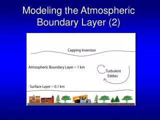
Refractivity in the Coastal Atmospheric Boundary Layer. Stephen Burk and Tracy Haack Naval Research Laboratory Monterey, CA. Strength ( M). Height. top. Thickness (= top-base). base. Modified Refractivity, M. Refractivity in the Coastal Atmospheric Boundary Layer. . Q. Height.

E N D
Refractivity in the Coastal Atmospheric Boundary Layer Stephen Burk and Tracy Haack Naval Research Laboratory Monterey, CA
Strength (M) Height top Thickness (= top-base) base Modified Refractivity, M Refractivity in the Coastal Atmospheric Boundary Layer Q Height Potential Temperature & Specific Humidity
COAMPSTM 27km grid SAUDI ARABIA INDIA Cook & Burk, 1992, BLM, 58, 151-159. Burk & Thompson, 1997, JAM, 36, 22-31. Haack & Burk, 2001, JAM, 40, 673-687. Burk, Haack, Rogers, & Wagner, 2003, JAM, 349-367.
Wallops 2000 EM Propagation Field Experiment from NSWCDD/TR-01/132
DMDZ/THETA Height (m) COAMPSTM Wallops Island DTG: 10-12 Apr 2000 Triple nest: 27-9-3 km Vertical: 40 levels SST/SLP 10-m Winds/SLP x = 3 km x = 27 km
April 10, 2000 1200 UTC April 12, 2000 1200 UTC April 11, 2000 1200 UTC
Dots = COAMPSTM forecast values EDH(m) RH(%) Ta T(0C) IR U(m/s) Obs from Davidson, NPS
Wallops * Norfolk COAMPSTM SST and Ground Temperature * 284 297 3 am LT 10 Apr 2000
20 20 0 0 0 -20 0 0 40 0 0 40 -20 20 0 20 60 60 COAMPSTM Sensible Heat Flux (W/m2); near surface streamlines 11 Apr 2000 3 am LT 3 pm LT
2 6 10 8 4 12 4 24 28 COAMPSTM Evaporation Duct Height (m) 11 Apr 2000 3 am LT 3 pm LT
Strength (M) Height top base Modified Refractivity, M Animation of two 24h COAMPSTM forecasts of: 40m(shaded); 50m streamlines; & dM/dz = 0 isosurface (white) hourly fields from 00 UTC 11 Apr- 2300 UTC 12 Apr 2000
North South 1 km 0 Horizontal: Evaporation Duct Height (shaded) & Streamlines Vertical: Potential Temperature (shaded & contoured) “Clouds”: Trapping Layer (DMDZ=0 isosurface)
(a) (b) M Crossection M Crossection Shaded with dM/dz (c) Looking toward SE across Tidewater Peninsula Red Isosurface dM/dz = 157 M-units/km subrefraction White isosurface dM/dz = 0 M-units/km trapping layer 1800 UTC 12 Apr 2000 COAMPSTM
1800 UTC 12 Apr 2000 COAMPSTM Mixing Ratio (g/kg), Shaded; Potential Temperature (K),contoured
Duct parameters from COAMPSTM 1800 UTC 12 Apr 2000 Wallops Island 500 400 300 18 15 300 200 12 200 9 100 100 6 0 3 0 0 Duct Base Height (m) Duct Thickness (m) Duct Strength (M-units)
Summary • COAMPSTM forecasts both evaporation ducts and elevated and/or • surface based ducts • To date, most modeling studies of refractivity/propagation have focused on • subsidence dominated, strongly capped BL’s (e.g., CA coast in summer; • Persian Gulf) • Intensive Observation Periods of the Wallops-2000 propagation field experiment • are addressed here using COAMPSTM at high resolution. Model refractivity • will be inserted into propagation codes for comparison with prop measurements. • New insights into refractivity structure in frontal regions are emerging • Accurate forecasting of major synoptic features (e.g., frontal boundaries) can be • of greater importance than extremely high model resolution in defining local • refractive structure/ EM propagation conditions. Mesoscale ensembles may • be very useful in this context.