Download
1 / 36
360 likes | 530 Vues
B.V. Jackson, and P.P. Hick, A. Buffington, J.M. Clover, N. Amirbekian Center for Astrophysics and Space Sciences, University of California at San Diego, LaJolla, CA, USA. and. D.B. Reisenfeld Department of Physics and Astronomy, University of Montana, Missoula, MT, USA. Masayoshi.

E N D
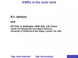
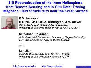
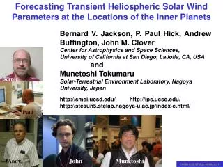
B.V. Jackson, and P.P. Hick, A. Buffington, J.M. Clover, N. Amirbekian Center for Astrophysics and Space Sciences, University of California at San Diego, LaJolla, CA, USA and D.B. Reisenfeld Department of Physics and Astronomy, University of Montana, Missoula, MT, USA Masayoshi http://smei.ucsd.edu/ http://ips.ucsd.edu/
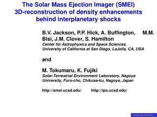
Introduction: The Digital Analysis: 3-D Heliospheric Tomography – (a fit to data) (Time-dependent view from a single observer location) The Data Sets: IPS (Intestellar Scintillation), SMEI (the Solar Mass Ejection Imager) The Motive: Voyager Solar Wind Measurements, 3-D Interstellar boundary This Project: An inner heliospheric boundary
STELab IPS Heliospheric Analyses DATA STELab IPS array near Fujioperating at 327 MHz
Current STELab IPS Heliospheric Analyses New STELab IPS array at Toyokawa - photo February 17, 2007 (new 327 MHz array now operates)
Scintillation Level Heliospheric Analysis Jackson, B.V., et al., 2008, Adv. in Geosciences , 21, 339-366. Intensity interplanetary scintillation (IPS) g-levels. STELab IPS IPS line-of-sight response g = m/<m>
Heliospheric 3-D Reconstruction Jackson, B.V., et al., 2008, Adv. in Geosciences , 21, 339-366. The outward-flowing solar wind structure follows very specific physics as it moves outward from the Sun LOS Weighting
Heliospheric 3-D Reconstruction Jackson, B.V., et al., 2008, Adv. in Geosciences , 21, 339-366. Line of sight “crossed” components on a reference surface. Projections on the reference surface are shown. These weighted components are inverted to provide the time-dependent tomographic reconstruction. 13 July 2000 14 July 2000
Jackson, B.V., et al., 2008, Adv. in Geosciences , 21, 339-366. The UCSD 3D-reconstruction program The “traceback matrix”(any solar-wind model works)In the traceback matrix the location of the upper level data point (starred) is an interpolation in x of Δx2 and the unit x distance – Δx3 distance or (1 – Δx3). Similarly, the value of Δt at the starred point is interpolated by the same spatial distance. Each 3D traceback matrix contains a regular grid of values ΣΔx, ΣΔy, ΣΔt, ΣΔv, and ΣΔm that locates the origin of each point in the grid at each time and its change in velocity and density from the heliospheric model.
http://ips.ucsd.edu/ UCSD time-dependent IPS Web forecast Velocity model time-series G-level sky map Real-time tomographic analysis of the solar wind on April 29-30, 2004 showing a halo CME response in the interplanetary medium. Web Analysis Runs Automatically Using Linux on a P.C.
Tokumaru, M., et al., 2010, J. Geophys Res. (in press). “Solar cycle evolution of the solar wind speed from 1985-2008” (part of the result is shown here). The recently past solar minimum is pretty special in that there is a large variation of solar wind speed over solar latitude.
UCSD time-dependent IPS Velocity and density analysis (also at the CCMC) Density ecliptic cut Velocity ecliptic cut Tomographic analysis of the solar wind for Carrington rotation 2085 (2009/06/26 – 2009/07/23).
UCSD time-dependent IPS Velocity and density analysis (also at the CCMC) Density meridional cut Velocity meridional cut Tomographic analysis of the solar wind for Carrington rotation 2085 (2009/06/26 – 2009/07/23).
UCSD time-dependent IPS Velocity and density analysis (also at the CCMC) Density remote-observer view Velocity remote-observer view Tomographic analysis of the solar wind for Carrington rotation 2085 (2009/06/26 – 2009/07/23).
The Solar Mass Ejection Imager (SMEI) Mission -- Journal Article B. V. Jackson, A. Buffington, P. P. Hick Center for Astrophysics and Space Sciences, University of California at San Diego, LaJolla, CA. R.C. Altrock, S. Figueroa, P.E. Holladay, J.C. Johnston, S.W. Kahler, J.B. Mozer, S. Price,R.R. Radick, R. Sagalyn, D. Sinclair Air Force Research Laboratory/Space Vehicles Directorate (AFRL/VS), Hanscom AFB, MA G.M. Simnett, C.J. Eyles, M.P. Cooke, S.J. Tappin School of Physics and Space Research, University of Birmingham, UK T. Kuchar, D. Mizuno, D.F.Webb ISR, Boston College, Newton Center, MA P.A. Anderson Boston University, Boston, MA S.L. Keil National Solar Observatory, Sunspot, NM R.E. Gold Johns Hopkins University/Applied Physics Laboratory, Laurel, MD N.R. Waltham Space Science Dept., Rutherford-Appleton Laboratory, Chilton, UK The Coriolis spacecraft at Vandenberg prior to flight. The SMEI baffles are circled. The large NRL radiometer Windsat is on the top of the spacecraft.
Data!! Lots of Data!! <---Sun C1 C2 C3 Sun | V Simultaneous images from the three SMEI cameras.
Frame Composite for Aitoff Map Blue = Cam3; Green= Cam2; Red = Cam1 D290; 17 October 2003
SMEI first light composite image Composite all-sky map Feb 2, 2003 from the three SMEI cameras.
Images from the 3-D reconstructions 26 May – 05 June 2003, (May 28 ‘Halo’ CME)
Jackson, B.V., et al., 2008, J. Geophys Res., 113, A00A15, doi:10.1029/2008JA013224 Other 2003 May 27-28 CME events SMEI density 3D reconstruction of the 28 May 2003 halo CME as viewed from 15º above the ecliptic plane about 30º east of the Sun-Earth line. SMEI density (remote observer view) of the 28 May 2003 halo CME
Jackson, B.V., et al., 2008, J. Geophys Res., 113, A00A15, doi:10.1029/2008JA013224 SMEI & IPS 27-28 May 2003 CME event period IPS Velocity and SMEI proton density reconstruction of the 27-28 May 2003 halo CME sequence. Reconstructed and Windin-situ densities are compared with over one Carrington rotation.
26 April 2008 CME/ICME SMEI difference image LASCO SMEI SMEI 3-D reconstruction of the 26 April 2008 CME as it arrives at Earth and the STEREO-B spacecraft.
26-29 April 2008 period SMEI SMEI ENLIL SMEI proton density 3-D reconstruction of the 26 April 2008 CME as it arrives at Earth and the STEREO spacecraft compared with ENLIL.
27-30 April 2008 period SMEI 3-D Reconstructed densities (most of the ICME density is North and East of STEREO-B.
27-30 April 2008 period SMEI/STEREO-B density SMEI/STEREO-B density IPS/STEREO-B velocity 3-D Reconstructed and STEREO-Bin-situ densities and velocities.
To go farther distances from the Sun: The best procedure is to obtain an inner heliosphere boundary of physical parameters, and using the best physics, extrapolate this outward to the largest distance possible. We expect some variation in the inner solar wind will be manifest in Voyager or ENA flux observed at large distances from the Sun. In this way one hopes to learn more about the physics and the digital process that provides this extrapolation to the observed distant heliosphere.
4065 eV In addition: 2008 2558 eV 1726 eV 2009 North ecliptic pole heliospheric 0.5 AU pressure. North ecliptic pole ENAs (IBEX launch 2008 October 19) (Dan Reisenfeld)
Carrington Rotations 2084-2085 Speed at 0.5 AU (ecliptic coordinates).
Carrington Rotations 2084-2085 Density at 0.5 AU (ecliptic coordinates).
Carrington Rotations 2084-2085 Pressure at 0.5 AU (ecliptic coordinates).
2008 2009 North ecliptic pole heliospheric 0.5 AU density and velocity from the IPS density (normalized to 1 AU).
4065 eV 2008 2558 eV 1726 eV 2009 North ecliptic pole heliospheric 0.5 AU pressure. North ecliptic pole ENAs (IBEX launch 2008 October 19) (Dan Reisenfeld)
Summary: The analysis of IPS data provides low-resolution global measurements of density and velocity with a time cadence of about a day. There are several data sources (IPS, SMEI), but the most long-term and substantiated (that also measure velocity globally) are the STELab arrays in Japan. Accurate observations of inner heliosphere parameters coupled withthe best physicscan extrapolate these outward to the interstellar boundary.