Download
1 / 24
240 likes | 361 Vues
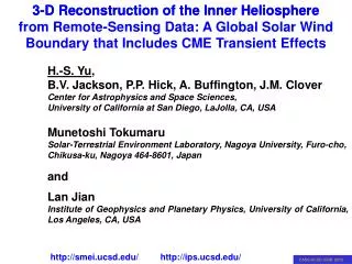
3-D Reconstruction of the Inner Heliosphere from Remote-Sensing Data: A Global Solar Wind Boundary that Includes CME Transient Effects. H.-S. Yu , B.V. Jackson, P.P. Hick, A. Buffington, J.M. Clover Center for Astrophysics and Space Sciences,

E N D
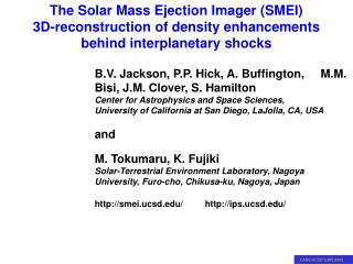
3-D Reconstruction of the Inner Heliosphere from Remote-Sensing Data: A Global Solar Wind Boundary that Includes CME Transient Effects H.-S. Yu, B.V. Jackson, P.P. Hick, A. Buffington, J.M. Clover Center for Astrophysics and Space Sciences, University of California at San Diego, LaJolla, CA, USA Munetoshi Tokumaru Solar-Terrestrial Environment Laboratory, Nagoya University, Furo-cho, Chikusa-ku, Nagoya 464-8601, Japan and Lan Jian Institute of Geophysics and Planetary Physics, University of California, Los Angeles, CA, USA Masayoshi http://smei.ucsd.edu/ http://ips.ucsd.edu/
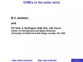
Introduction: The Motive: A 3-D Boundary for MHD models The Analysis: 3-D Heliospheric Tomography – (a fit to data) (Time-dependent view from a single observer location) The Data Sets: STELab IPS This Project: The analysis that includes in-situ data and magnetic field trace to near the solar surface.
DATA STELab IPS Heliospheric Analyses IPS line-of-sight response STELab IPS array near Mt. Fuji STELab IPS array systems
Density Turbulence • Scintillation index, m, is a measure of level of turbulence • Normalized Scintillation index, g = m(R) / <m(R)> • g > 1 enhancement in Ne • g 1 ambient level of Ne • g < 1 rarefaction in Ne (CourtesyofP.K.Manoharan) A scintillation enhancement with respect to the ambient wind identifies the presence of a region of increased turbulence/density and a possible CME along the line-of-sight to the radio source.
Current STELab IPS Heliospheric Analyses New STELab IPS array at Toyokawa - photo February 17, 2007 (array now operates well – year-round operation to provide scintillation-level measurements)
Tokumaru, M., et al., 2010, J. Geophys Res., 115, A04102. “Corotating” analysis since 1985 “Solar cycle evolution of the solar wind speed from 1985-2008” (part of the result is shown here). The recently past solar minimum is pretty special in that there is a large variation of solar wind speed over solar latitude.
UCSD Heliospheric 3-D Reconstruction Jackson, B.V., et al., 2008, Adv. in Geosciences, 21, 339 The outward-flowing solar wind structure follows very specific physics as it moves outward from the Sun. We assume conservation of mass and mass flux. LOS Weighting
Jackson, B.V., et al., 2008, Adv. in Geosciences, 21, 339. The UCSD 3D-reconstruction program The “traceback matrix”(any solar wind model works)In the traceback matrix the location of the upper level data point (starred) is an interpolation in x of Δx2 and the unit x distance – Δx3 distance or (1 – Δx3). Similarly, the value of Δt at the starred point is interpolated by the same spatial distance. Each 3D traceback matrix contains a regular grid of values ΣΔx, ΣΔy, ΣΔt, ΣΔv, and ΣΔm that locates the origin of each point in the grid at each time and its change in velocity and density from the heliospheric model.
Heliospheric 3-D Reconstruction Jackson, B.V., et al., 2008, Adv. in Geosciences, 21, 339. Line of sight “crossed” components on a reference surface. Projections on the reference surface are shown. These weighted components are inverted on this 2D surface to provide the time-dependent tomographic reconstruction. 13 July 2000 14 July 2000
Jackson, B.V., et al., 2010,Solar Phys., 265, 245-256. IPS line-of-sight response Jackson, B.V., et al., 2008, Adv. in Geosciences, 21, 339. The inclusion of in-situ data provides a more stable 3D reconstruction solution globally, and allows a better interpolation across time intervals without much remote-sensing data. Innovation STELab IPS * 13 July 2000 Inclusion of in-situ measurements into the 3D-reconstructions
IPS C.A.T. Analysis Jackson, B.V., et al., 2002, Solar Wind 10, 31 Bastille Day Event 14 July 2000
IPS C.A.T. Analysis Jackson, B.V., et al., 2002, Solar Wind 10, 31 Bastille Day Event 14 July 2000
Zhao, X. P. and Hoeksema, J. T., 1995, J. Geophys. Res., 100 (A1), 19. http://ips.ucsd.edu/ Magnetic Field Extrapolation Dunn et al., 2005, Solar Physics 227: 339–353. • Inner region: the CSSS model calculates the magnetic field usingphotospheric measurements and a horizontal current model. 2. Middle region: the CSSS model opens the field lines. In the outer region. 3. Outer region: the UCSD tomography convects the magnetic field along velocity flow lines. Jackson, B.V., et al., 2012, Adv. in Geosciences (in press)
IPS C.A.T. Analysis Dunn, T.J., et al., 2005, Solar Phys., 227, 339 Potential field modeling added
To Make a 3D-MHD Boundary Time-Dependent Velocity at 0.25 AU IHG Coordinates ACE in-situ Measurement Inclusion
To Make a 3D-MHD Boundary Time-Dependent Density at 0.25 AU IHG Coordinates ACE in-situ Measurement Inclusion
To Make a 3D-MHD Boundary Time-Dependent Radial Field at 0.25 AU, IHG Coordinates ACE in-situ Measurement Inclusion
To Make a 3D-MHD Boundary Time-Dependent Tangential Field at 0.25 AU IHG Coordinates ACE in-situ Measurement Inclusion
Heliospheric 3D-reconstructions Jackson, B.V., et al., 2010,Solar Phys., 265, 245-256. Lan Jian CCMC Study In-SituTomographic analysis
Heliospheric 3D-reconstructions Jackson, B.V., et al., 2010,Solar Phys., 265, 245-256. Lan Jian CCMC Study In-SituTomographic analysis
Heliospheric 3D-reconstructions Jackson, B.V., et al., 2010,Solar Phys., 265, 245-256. Lan Jian CCMC Study In-SituTomographic analysis
Heliospheric 3D-reconstructions Jackson, B.V., et al., 2010,Solar Phys., 265, 245-256. Lan Jian CCMC Study In-SituTomographic analysis
Magnetic Field Traceback Traceback Matrix Time-Dependent Radial Field at 0.25 AU, IHG Coordinates
Summary: The analysis of IPS data provides low-resolution global measurements of density and velocity with a time cadence of one day for both density and velocity, and slightly longer cadences for some magnetic field components. There are several data sources (IPS, SMEI), but the most long-term and substantiated data source (that also measures velocity globally) is IPS data from the STELab arrays in Japan. Accurate observations of inner heliosphere parameters coupled withthe best physicscan extrapolate these outward to Earth or the interstellar boundary.