Download
1 / 112
1.12k likes | 1.19k Vues
Explore the evolution of dense linear algebra software & its key computational patterns. Learn about BLAS libraries, parallel matrix multiplication, & achieving lower communication-bound. Dive into eigenvalues, singular values, and matrix structures.

E N D
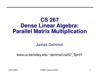
CS 267Dense Linear Algebra:History and Structure,Parallel Matrix Multiplication James Demmel www.cs.berkeley.edu/~demmel/cs267_Spr13 CS267 Lecture 11
Quick review of earlier lecture • What do you call • A program written in PyGAS, a Global Address Space language based on Python… • That uses a Monte Carlo simulation algorithm to approximate π … • That has a race condition, so that it gives you a different funny answer every time you run it? Monte - π - thon CS267 Lecture 11
Outline • History and motivation • Lower bound on communication • Structure of the Dense Linear Algebra motif • What does A\b do? • Parallel Matrix-matrix multiplication • Attaining the lower bound • Proof of the lower bound • Parallel Gaussian Elimination (next time) CS267 Lecture 11
Outline • History and motivation • Lower bound on communication • Structure of the Dense Linear Algebra motif • What does A\b do? • Parallel Matrix-matrix multiplication • Attaining the lower bound • Proof of the lower bound • Parallel Gaussian Elimination (next time) CS267 Lecture 11
Motifs The Motifs (formerly “Dwarfs”) from “The Berkeley View” (Asanovic et al.) Motifs form key computational patterns
What is dense linear algebra? • Not just matmul! • Linear Systems: Ax=b • Least Squares: choose x to minimize ||Ax-b||2 • Overdetermined or underdetermined • Unconstrained, constrained, weighted • Eigenvalues and vectors of Symmetric Matrices • Standard (Ax = λx), Generalized (Ax=λBx) • Eigenvalues and vectors of Unsymmetric matrices • Eigenvalues, Schur form, eigenvectors, invariant subspaces • Standard, Generalized • Singular Values and vectors (SVD) • Standard, Generalized • Different matrix structures • Real, complex; Symmetric, Hermitian, positive definite; dense, triangular, banded … • Level of detail • Simple Driver (“x=A\b”) • Expert Drivers with error bounds, extra-precision, other options • Lower level routines (“apply certain kind of orthogonal transformation”, matmul…) CS267 Lecture 11
A brief history of (Dense) Linear Algebra software (1/7) • In the beginning was the do-loop… • Libraries like EISPACK (for eigenvalue problems) • Then the BLAS (1) were invented (1973-1977) • Standard library of 15 operations (mostly) on vectors • “AXPY” ( y = α·x + y ), dot product, scale (x = α·x ), etc • Up to 4 versions of each (S/D/C/Z), 46 routines, 3300 LOC • Goals • Common “pattern” to ease programming, readability • Robustness, via careful coding (avoiding over/underflow) • Portability + Efficiency via machine specific implementations • Why BLAS 1 ? They do O(n1) ops on O(n1) data • Used in libraries like LINPACK (for linear systems) • Source of the name “LINPACK Benchmark” (not the code!) CS267 Lecture 11
Current Records for Solving Dense Systems (11/2012) • Linpack Benchmark • Fastest machine overall (www.top500.org) • Cray TITAN (Oak Ridge National Lab) • 17.6 Petaflops out of 27.1 Petaflops peak • 18,688 compute nodes, each with 16 core Opteron • and Nvidia Tesla K20 GPU • 299,008 Opteron cores • 710 Terabytes memory • 8.2 MW of power • Historical data (www.netlib.org/performance) • Palm Pilot III • 1.69 Kiloflops • n = 100 CS267 Lecture 11
A brief history of (Dense) Linear Algebra software (2/7) • But the BLAS-1 weren’t enough • Consider AXPY ( y = α·x + y ): 2n flops on 3n read/writes • Computational intensity = (2n)/(3n) = 2/3 • Too low to run near peak speed (read/write dominates) • Hard to vectorize (“SIMD’ize”) on supercomputers of the day (1980s) • So the BLAS-2 were invented (1984-1986) • Standard library of 25 operations (mostly) on matrix/vector pairs • “GEMV”: y = α·A·x + β·x, “GER”: A = A + α·x·yT, x = T-1·x • Up to 4 versions of each (S/D/C/Z), 66 routines, 18K LOC • Why BLAS 2 ? They do O(n2) ops on O(n2) data • So computational intensity still just ~(2n2)/(n2) = 2 • OK for vector machines, but not for machine with caches CS267 Lecture 11
A brief history of (Dense) Linear Algebra software (3/7) • The next step: BLAS-3 (1987-1988) • Standard library of 9 operations (mostly) on matrix/matrix pairs • “GEMM”: C = α·A·B + β·C, C = α·A·AT + β·C, B = T-1·B • Up to 4 versions of each (S/D/C/Z), 30 routines, 10K LOC • Why BLAS 3 ? They do O(n3) ops on O(n2) data • So computational intensity (2n3)/(4n2) = n/2 – big at last! • Good for machines with caches, other mem. hierarchy levels • How much BLAS1/2/3 code so far (all at www.netlib.org/blas) • Source: 142 routines, 31K LOC, Testing: 28K LOC • Reference (unoptimized) implementation only • Ex: 3 nested loops for GEMM • Lots more optimized code (eg Homework 1) • Motivates “automatic tuning” of the BLAS • Part of standard math libraries (eg AMD ACML, Intel MKL) CS267 Lecture 11
A brief history of (Dense) Linear Algebra software (4/7) • LAPACK – “Linear Algebra PACKage” - uses BLAS-3 (1989 – now) • Ex: Obvious way to express Gaussian Elimination (GE) is adding multiples of one row to other rows – BLAS-1 • How do we reorganize GE to use BLAS-3 ? (details later) • Contents of LAPACK (summary) • Algorithms that are (nearly) 100% BLAS 3 • Linear Systems: solve Ax=b for x • Least Squares: choose x to minimize ||Ax-b||2 • Algorithms that are only 50% BLAS 3 • Eigenproblems: Findland x where Ax = l x • Singular Value Decomposition (SVD) • Generalized problems (eg Ax = l Bx) • Error bounds for everything • Lots of variants depending on A’s structure (banded, A=AT, etc) • How much code? (Release 3.3, Nov 2010) (www.netlib.org/lapack) • Source: 1586 routines, 500K LOC, Testing: 363K LOC • Ongoing development (at UCB and elsewhere) (class projects!) • Up to release 3.4.1 in Apr 2012 CS267 Lecture 11
A brief history of (Dense) Linear Algebra software (5/7) • Is LAPACK parallel? • Only if the BLAS are parallel (possible in shared memory) • ScaLAPACK – “Scalable LAPACK” (1995 – now) • For distributed memory – uses MPI • More complex data structures, algorithms than LAPACK • Only (small) subset of LAPACK’s functionality available • Details later (class projects!) • All at www.netlib.org/scalapack CS267 Lecture 11
Success Stories for Sca/LAPACK (6/7) • Widely used • Adopted by Mathworks, Cray, Fujitsu, HP, IBM, IMSL, Intel, NAG, NEC, SGI, … • 7.5M webhits/year @ Netlib (incl. CLAPACK, LAPACK95) • New Science discovered through the solution of dense matrix systems • Nature article on the flat universe used ScaLAPACK • Other articles in Physics Review B that also use it • 1998 Gordon Bell Prize • www.nersc.gov/news/reports/newNERSCresults050703.pdf Cosmic Microwave Background Analysis, BOOMERanG collaboration, MADCAP code (Apr. 27, 2000). ScaLAPACK CS267 Lecture 11
A brief future look at (Dense) Linear Algebra software (7/7) • PLASMA and MAGMA (now) • Ongoing extensions to Multicore/GPU/Heterogeneous • Can one software infrastructure accommodate all algorithms and platforms of current (future) interest? • How much code generation and tuning can we automate? • Details later (Class projects!) (icl.cs.utk.edu/{plasma,magma}) • Other related projects • BLAST Forum (www.netlib.org/blas/blast-forum) • Attempt to extend BLAS to other languages, add some new functions, sparse matrices, extra-precision, interval arithmetic • Only partly successful (extra-precise BLAS used in latest LAPACK) • FLAME (z.cs.utexas.edu/wiki/flame.wiki/FrontPage) • Formal Linear Algebra Method Environment • Attempt to automate code generation across multiple platforms CS267 Lecture 11
Back to basics: Why avoiding communication is important (1/3) Algorithms have two costs: Arithmetic (FLOPS) Communication: moving data between levels of a memory hierarchy (sequential case) processors over a network (parallel case). CPU Cache CPU DRAM CPU DRAM DRAM CPU DRAM CPU DRAM CS267 Lecture 11
Why avoiding communication is important (2/3) communication • Time_per_flop << 1/ bandwidth << latency • Gaps growing exponentially with time 59% • Goal : organize linear algebra to avoid communication • Between all memory hierarchy levels • L1 L2 DRAM network, etc • Notjust hiding communication (overlap with arith) (speedup 2x ) • Arbitrary speedups possible • Minimize communication to save time • Running time of an algorithm is sum of 3 terms: • # flops * time_per_flop • # words moved / bandwidth • # messages * latency CS267 Lecture 11 02/26/2013
Why Minimize Communication? (3/3) Source: John Shalf, LBL
Why Minimize Communication? (3/3) Minimize communication to save energy Source: John Shalf, LBL
Goal: Organize Linear Algebra to Avoid Communication • Between all memory hierarchy levels • L1 L2 DRAM network, etc • Notjust hiding communication (overlap with arithmetic) • Speedup 2x • Arbitrary speedups/energy savings possible • Later: Same goal for other computational patterns • Lots of open problems 02/26/2013
Review: Naïve Sequential MatMul: C = C + A*B for i = 1 to n {read row i of A into fast memory, n2 reads} for j = 1 to n {read C(i,j) into fast memory, n2 reads} {read column j of B into fast memory, n3 reads} for k = 1 to n C(i,j) = C(i,j) + A(i,k) * B(k,j) {write C(i,j) back to slow memory, n2 writes} n3 + O(n2) reads/writes altogether A(i,:) C(i,j) C(i,j) B(:,j) = + * 02/26/2013 CS267 Lecture 11
Less Communication with Blocked Matrix Multiply • … Break Anxn, Bnxn, Cnxn into bxb blocks labeled A(i,j), etc • … b chosen so 3 bxb blocks fit in cache • for i = 1 to n/b, for j=1 to n/b, for k=1 to n/b • C(i,j) = C(i,j) + A(i,k)·B(k,j) … b x b matmul, 4b2 reads/writes • (n/b)3 · 4b2 = 4n3/b reads/writes altogether • Minimized when 3b2 = cache size = M, yielding O(n3/M1/2) reads/writes • What if we had more levels of memory? (L1, L2, cache etc)? • Would need 3 more nested loops per level Blocked Matmul C = A·B explicitly refers to subblocks of A, B and C of dimensions that depend on cache size 02/26/2013 CS267 Lecture 11
Blocked vs Cache-Oblivious Algorithms … Break Anxn, Bnxn, Cnxn into bxb blocks labeled A(i,j), etc … b chosen so 3 bxb blocks fit in cache for i = 1 to n/b, for j=1 to n/b, for k=1 to n/b C(i,j) = C(i,j) + A(i,k)·B(k,j) … b x b matmul … another level of memory would need 3 more loops • Cache-oblivious Matmul C = A·B is independent of cache Function C = RMM(A,B) … R for recursive If A and B are 1x1 C = A · B else … Break Anxn, Bnxn, Cnxn into (n/2)x(n/2) blocks labeled A(i,j), etc for i = 1 to 2, for j = 1 to 2, for k = 1 to 2 C(i,j) = C(i,j) + RMM( A(i,k), B(k,j) ) … n/2 x n/2 matmul Blocked Matmul C = A·B explicitly refers to subblocks of A, B and C of dimensions that depend on cache size CS267 Lecture 11 02/26/2013
Communication Lower Bounds: Prior Work on Matmul • Parallel case on P processors: • Let M be memory per processor; assume load balanced • Lower bound on #words moved = (n3 /(p · M1/2 )) [Irony, Tiskin, Toledo, 04] • If M = 3n2/p (one copy of each matrix), then lower bound = (n2 /p1/2 ) • Attained by SUMMA, Cannon’s algorithm 02/26/2013 • Assume n3 algorithm (i.e. not Strassen-like) • Sequential case, with fast memory of size M • Lower bound on #words moved to/from slow memory = (n3 / M1/2) [Hong, Kung, 81] • Attained using blocked or cache-oblivious algorithms CS267 Lecture 11
New lower bound for all “direct” linear algebra • Let M = “fast” memory size per processor • = cache size (sequential case) or O(n2/p) (parallel case) • #flops = number of flops done per processor • #words_moved per processor = (#flops / M1/2) • #messages_sent per processor = (#flops / M3/2) • Holds for • Matmul, BLAS, LU, QR, eig, SVD, tensor contractions, … • Some whole programs (sequences of these operations, no matter how they are interleaved, eg computing Ak) • Dense and sparse matrices (where #flops << n3 ) • Sequential and parallel algorithms • Some graph-theoretic algorithms (eg Floyd-Warshall) • Proof later 02/26/2013 CS267 Lecture 11
New lower bound for all “direct” linear algebra • Let M = “fast” memory size per processor • = cache size (sequential case) or O(n2/p) (parallel case) • #flops = number of flops done per processor • #words_moved per processor = (#flops / M1/2) • #messages_sent per processor = (#flops / M3/2) SIAM Linear Algebra Prize, 2012 • Sequential case, dense n x n matrices, so O(n3) flops • #words_moved = (n3/ M1/2 ) • #messages_sent = (n3/ M3/2 ) • Parallel case, dense n x n matrices • Load balanced, so O(n3/p) flops processor • One copy of data, load balanced, so M = O(n2/p) per processor • #words_moved = (n2/ p1/2 ) • #messages_sent = ( p1/2 ) 02/26/2013 CS267 Lecture 11
Can we attain these lower bounds? • Do conventional dense algorithms as implemented in LAPACK and ScaLAPACK attain these bounds? • Mostly not yet • If not, are there other algorithms that do? • Yes • Goals for algorithms: • Minimize #words_moved • Minimize #messages_sent • Need new data structures • Minimize for multiple memory hierarchy levels • Cache-oblivious algorithms would be simplest • Fewest flops when matrix fits in fastest memory • Cache-oblivious algorithms don’t always attain this • Attainable for nearly all dense linear algebra • Just a few prototype implementations so far (class projects!) • Only a few sparse algorithms so far (eg Cholesky) 02/26/2013 CS267 Lecture 11
Outline • History and motivation • Lower bound on communication • Structure of the Dense Linear Algebra motif • What does A\b do? • Parallel Matrix-matrix multiplication • Attaining the lower bound • Proof of the lower bound • Parallel Gaussian Elimination (next time) CS267 Lecture 11
What could go into the linear algebra motif(s)? For all linear algebra problems For all matrix/problem structures For all data types For all architectures and networks For all programming interfaces Produce best algorithm(s) w.r.t. performance and/or accuracy (including error bounds, etc) Need to prioritize, automate! CS267 Lecture 11
For all linear algebra problems:Ex: LAPACK Table of Contents • Linear Systems • Least Squares • Overdetermined, underdetermined • Unconstrained, constrained, weighted • Eigenvalues and vectors of Symmetric Matrices • Standard (Ax = λx), Generalized (Ax=λBx) • Eigenvalues and vectors of Unsymmetric matrices • Eigenvalues, Schur form, eigenvectors, invariant subspaces • Standard, Generalized • Singular Values and vectors (SVD) • Standard, Generalized • Level of detail • Simple Driver • Expert Drivers with error bounds, extra-precision, other options • Lower level routines (“apply certain kind of orthogonal transformation”) CS267 Lecture 11
What does A\b do? What could it do?Ex: LAPACK Table of Contents • BD – bidiagonal • GB – general banded • GE – general • GG – general , pair • GT – tridiagonal • HB – Hermitian banded • HE – Hermitian • HG – upper Hessenberg, pair • HP – Hermitian, packed • HS – upper Hessenberg • OR – (real) orthogonal • OP – (real) orthogonal, packed • PB – positive definite, banded • PO – positive definite • PP – positive definite, packed • PT – positive definite, tridiagonal • SB – symmetric, banded • SP – symmetric, packed • ST – symmetric, tridiagonal • SY – symmetric • TB – triangular, banded • TG – triangular, pair • TP – triangular, packed • TR – triangular • TZ – trapezoidal • UN – unitary • UP – unitary packed CS267 Lecture 11
What does A\b do? What could it do?Ex: LAPACK Table of Contents • BD – bidiagonal • GB – general banded • GE – general • GG – general , pair • GT – tridiagonal • HB – Hermitian banded • HE – Hermitian • HG – upper Hessenberg, pair • HP – Hermitian, packed • HS – upper Hessenberg • OR – (real) orthogonal • OP – (real) orthogonal, packed • PB – positive definite, banded • PO – positive definite • PP – positive definite, packed • PT – positive definite, tridiagonal • SB – symmetric, banded • SP – symmetric, packed • ST – symmetric, tridiagonal • SY – symmetric • TB – triangular, banded • TG – triangular, pair • TP – triangular, packed • TR – triangular • TZ – trapezoidal • UN – unitary • UP – unitary packed CS267 Lecture 11
What does A\b do? What could it do?Ex: LAPACK Table of Contents • BD – bidiagonal • GB – general banded • GE – general • GG – general, pair • GT – tridiagonal • HB – Hermitian banded • HE – Hermitian • HG – upper Hessenberg, pair • HP – Hermitian, packed • HS – upper Hessenberg • OR – (real) orthogonal • OP – (real) orthogonal, packed • PB – positive definite, banded • PO – positive definite • PP – positive definite, packed • PT – positive definite, tridiagonal • SB – symmetric, banded • SP – symmetric, packed • ST – symmetric, tridiagonal • SY – symmetric • TB – triangular, banded • TG – triangular, pair • TP – triangular, packed • TR – triangular • TZ – trapezoidal • UN – unitary • UP – unitary packed CS267 Lecture 11
What does A\b do? What could it do?Ex: LAPACK Table of Contents • BD – bidiagonal • GB – general banded • GE – general • GG – general, pair • GT – tridiagonal • HB – Hermitian banded • HE – Hermitian • HG – upper Hessenberg, pair • HP – Hermitian, packed • HS – upper Hessenberg • OR – (real) orthogonal • OP – (real) orthogonal, packed • PB – positive definite, banded • PO – positive definite • PP – positive definite, packed • PT – positive definite, tridiagonal • SB – symmetric, banded • SP – symmetric, packed • ST – symmetric, tridiagonal • SY – symmetric • TB – triangular, banded • TG – triangular, pair • TP – triangular, packed • TR – triangular • TZ – trapezoidal • UN – unitary • UP – unitary packed CS267 Lecture 11
What does A\b do? What could it do?Ex: LAPACK Table of Contents • BD – bidiagonal • GB – general banded • GE – general • GG – general, pair • GT – tridiagonal • HB – Hermitian banded • HE – Hermitian • HG – upper Hessenberg, pair • HP – Hermitian, packed • HS – upper Hessenberg • OR – (real) orthogonal • OP – (real) orthogonal, packed • PB – positive definite, banded • PO – positive definite • PP – positive definite, packed • PT – positive definite, tridiagonal • SB – symmetric, banded • SP – symmetric, packed • ST – symmetric, tridiagonal • SY – symmetric • TB – triangular, banded • TG – triangular, pair • TP – triangular, packed • TR – triangular • TZ – trapezoidal • UN – unitary • UP – unitary packed CS267 Lecture 11
Organizing Linear Algebra – in books www.netlib.org/lapack www.netlib.org/scalapack gams.nist.gov www.netlib.org/templates www.cs.utk.edu/~dongarra/etemplates
Outline • History and motivation • Lower bound on communication • Structure of the Dense Linear Algebra motif • What does A\b do? • Parallel Matrix-matrix multiplication • Attaining the lower bound • Proof of the lower bound • Parallel Gaussian Elimination (next time) CS267 Lecture 11
Different Parallel Data Layouts for Matrices (not all!) 1) 1D Column Blocked Layout 2) 1D Column Cyclic Layout 4) Row versions of the previous layouts b 3) 1D Column Block Cyclic Layout Generalizes others 6) 2D Row and Column Block Cyclic Layout 5) 2D Row and Column Blocked Layout CS267 Lecture 11
Parallel Matrix-Vector Product • Compute y = y + A*x, where A is a dense matrix • Layout: • 1D row blocked • A(i) refers to the n by n/p block row that processor i owns, • x(i) and y(i) similarly refer to segments of x,y owned by i • Algorithm: • Foreach processor i • Broadcast x(i) • Compute y(i) = A(i)*x • Algorithm uses the formula y(i) = y(i) + A(i)*x = y(i) + Sj A(i,j)*x(j) P0 P1 P2 P3 x P0 P1 P2 P3 A(0) y A(1) A(2) A(3) CS267 Lecture 11
Matrix-Vector Product y = y + A*x • A column layout of the matrix eliminates the broadcast of x • But adds a reduction to update the destination y • A 2D blocked layout uses a broadcast and reduction, both on a subset of processors • sqrt(p) for square processor grid P0 P1 P2 P3 P0 P1 P2 P3 P4 P5 P6 P7 P8 P9 P10 P11 P12 P13 P14 P15 CS267 Lecture 11
Parallel Matrix Multiply • Computing C=C+A*B • Using basic algorithm: 2*n3 Flops • Variables are: • Data layout: 1D? 2D? Other? • Topology of machine: Ring? Torus? • Scheduling communication • Use of performance models for algorithm design • Message Time = “latency” + #words * time-per-word = a + n*b • Efficiency (in any model): • serial time / (p * parallel time) • perfect (linear) speedup efficiency = 1 CS267 Lecture 11
p0 p1 p2 p3 p4 p5 p6 p7 Matrix Multiply with 1D Column Layout • Assume matrices are n x n and n is divisible by p • A(i) refers to the n by n/p block column that processor i owns (similiarly for B(i) and C(i)) • B(i,j) is the n/p by n/p sublock of B(i) • in rows j*n/p through (j+1)*n/p - 1 • Algorithm uses the formula C(i) = C(i) + A*B(i) = C(i) + Sj A(j)*B(j,i) May be a reasonable assumption for analysis, not for code CS267 Lecture 11
Matrix Multiply: 1D Layout on Bus or Ring • Algorithm uses the formula C(i) = C(i) + A*B(i) = C(i) + Sj A(j)*B(j,i) • First consider a bus-connected machine without broadcast: only one pair of processors can communicate at a time (ethernet) • Second consider a machine with processors on a ring: all processors may communicate with nearest neighbors simultaneously CS267 Lecture 11
MatMul: 1D layout on Bus without Broadcast Naïve algorithm: C(myproc) = C(myproc) + A(myproc)*B(myproc,myproc) for i = 0 to p-1 for j = 0 to p-1 except i if (myproc == i) send A(i) to processor j if (myproc == j) receive A(i) from processor i C(myproc) = C(myproc) + A(i)*B(i,myproc) barrier Cost of inner loop: computation: 2*n*(n/p)2 = 2*n3/p2 communication: a + b*n2 /p CS267 Lecture 11
Naïve MatMul (continued) Cost of inner loop: computation: 2*n*(n/p)2 = 2*n3/p2 communication: a + b*n2 /p … approximately Only 1 pair of processors (i and j) are active on any iteration, and of those, only i is doing computation => the algorithm is almost entirely serial Running time: = (p*(p-1) + 1)*computation + p*(p-1)*communication 2*n3 + p2*a + p*n2*b This is worse than the serial time and grows with p. CS267 Lecture 11
Matmul for 1D layout on a Processor Ring • Pairs of adjacent processors can communicate simultaneously Copy A(myproc) into Tmp C(myproc) = C(myproc) + Tmp*B(myproc , myproc) for j = 1 to p-1 Send Tmp to processor myproc+1 mod p Receive Tmp from processor myproc-1 mod p C(myproc) = C(myproc) + Tmp*B( myproc-j mod p , myproc) • Same idea as for gravity in simple sharks and fish algorithm • May want double buffering in practice for overlap • Ignoring deadlock details in code • Time of inner loop = 2*(a + b*n2/p) + 2*n*(n/p)2 CS267 Lecture 11
Matmul for 1D layout on a Processor Ring • Time of inner loop = 2*(a + b*n2/p) + 2*n*(n/p)2 • Total Time = 2*n* (n/p)2 + (p-1) * Time of inner loop • 2*n3/p + 2*p*a + 2*b*n2 • (Nearly) Optimal for 1D layout on Ring or Bus, even with Broadcast: • Perfect speedup for arithmetic • A(myproc) must move to each other processor, costs at least (p-1)*cost of sending n*(n/p) words • Parallel Efficiency = 2*n3 / (p * Total Time) = 1/(1 + a * p2/(2*n3) + b * p/(2*n) ) = 1/ (1 + O(p/n)) • Grows to 1 as n/p increases (or a and b shrink) • But far from communication lower bound CS267 Lecture 11
Need to try 2D Matrix layout 1) 1D Column Blocked Layout 2) 1D Column Cyclic Layout 4) Row versions of the previous layouts b 3) 1D Column Block Cyclic Layout Generalizes others 6) 2D Row and Column Block Cyclic Layout 5) 2D Row and Column Blocked Layout CS267 Lecture 11
Summary of Parallel Matrix Multiply • SUMMA • Scalable Universal Matrix Multiply Algorithm • Attains communication lower bounds (within log p) • Cannon • Historically first, attains lower bounds • More assumptions • A and B square • P a perfect square • 2.5D SUMMA • Uses more memory to communicate even less • Parallel Strassen • Attains different, even lower bounds CS267 Lecture 11
SUMMA Algorithm • SUMMA = Scalable Universal Matrix Multiply • Presentation from van de Geijn and Watts • www.netlib.org/lapack/lawns/lawn96.ps • Similar ideas appeared many times • Used in practice in PBLAS = Parallel BLAS • www.netlib.org/lapack/lawns/lawn100.ps CS267 Lecture 11