Chapter 7: Matrix Algebra
Chapter 7: Matrix Algebra. (7.1) Matrix Arithmetic Matrix-Vector Multiplication Matrix-Matrix Multiplication (7.2) Applications. 1. (7.1) Matrix Arithmetic. Motivation. Recall once again Example 6.4: Initially our wetland is completely submerged and we know that every 10 years:

Chapter 7: Matrix Algebra
E N D
Presentation Transcript
Chapter 7: Matrix Algebra • (7.1) Matrix Arithmetic • Matrix-Vector Multiplication • Matrix-Matrix Multiplication • (7.2) Applications
1. (7.1) Matrix Arithmetic Motivation • Recall once again Example 6.4: • Initially our wetland is completely submerged and we know that every 10 years: • 5% of submerged wetlands become saturated wetland • 12% of saturated wetlands become dry • 100% of dry wetlands remain dry • We found the dynamic equations describing the change in composition each time step:
1. (7.1) Matrix Arithmetic Motivation • These equations are written succinctly as: • This last equation needs to be justified; that is, does matrix-vector multiplication accomplish here what we need? • In some sense, this is the wrong question- we should define some operation that does what we want; it just so turns out that the operation we want is what we call matrix multiplication.
1. (7.1) Matrix Arithmetic Motivation • So, let’s look once again at the dynamic equations and describe the operation that will do the job:
1. (7.1) Matrix Arithmetic Motivation • So, let’s look once again at the dynamic equations and describe the operation that will do the job: • Notice that we will need each entry of the first column of our transfer matrix to be multiplied by .
1. (7.1) Matrix Arithmetic Motivation • So, let’s look once again at the dynamic equations and describe the operation that will do the job: • And we need each entry of the second column of our transfer matrix to be multiplied by .
1. (7.1) Matrix Arithmetic Motivation • So, let’s look once again at the dynamic equations and describe the operation that will do the job: • Finally, we need each entry of the third column of our transfer matrix to be multiplied by .
1. (7.1) Matrix Arithmetic Motivation • So, we simply decide to let this: • mean this:
1. (7.1) Matrix Arithmetic Motivation • And we’ll have what we want: • But this is precisely the way that matrix-vector multiplication is defined! • If we look a bit closer, we can see two different points of view, or two different ways to think about this operation:
1. (7.1) Matrix Arithmetic Motivation • One way to think about this operation is as we just did- column-wise:
1. (7.1) Matrix Arithmetic Motivation • Another way to think about this operation is as rows acting on the column vector:
1. (7.1) Matrix Arithmetic Motivation • Both points of view yield the same result: • Different contexts will dictate which point of view one chooses to adopt. • Matrix-vector multiplication is a special case of matrix-matrix multiplication • We will soon need to use this more general operation • So, we now undertake a review of basic Matrix Arithmetic
1. (7.1) Matrix Arithmetic • Matrix Addition/Subtraction • This operation is defined just as we did for vectors; that is, addition and subtraction for matrices is componentwise • As before, this operation makes no sense for matrices with different dimensions • Example 7.1: A and M are the 2x3 matrices shown below. Add them. solution:
1. (7.1) Matrix Arithmetic • Matrix-Scalar Multiplication • This operation is also defined just as we did for vectors; that is, matrix-scalar multiplication is componentwise • Example:
1. (7.1) Matrix Arithmetic Matrix Multiplication • Matrix Multiplication is NOT what one might think! • It is NOT componentwise; let A and M be as before, then: • Moreover, dimension compatibility for matrix multiplication is NOT (necessarily) having the same dimensions; for instance: • Finally, matrix multiplication is NOT commutative:
1. (7.1) Matrix Arithmetic Matrix Multiplication • Before giving the definition of matrix multiplication, let’s first see an example where it is defined and how it is performed • Example 7.2: Let A and B be the following matrices. Find AB. Solution: Note: (2x3) (3x2) = (2x2) Note: In this case BA is defined (it will be a 3x3 matrix and it is NOT the same as AB), but this is NOT always the case!
1. (7.1) Matrix Arithmetic Matrix Multiplication • Definition: If A is an m × n matrix and B is an n × p matrix, then their product is an m × p matrix denoted by AB. If <AB>ij denotes the i,j entry of the product, then: • Note the dimension compatibility conditions for matrix multiplication:
1. (7.1) Matrix Arithmetic Matrix Multiplication • Heuristically, let A be 4x2 and B be 2x3. Then
1. (7.1) Matrix Arithmetic Matrix Multiplication • Let’s revisit example 7.2: Let A and B be the following matrices. This time, instead of finding AB, we calculate BA: Solution: Note: (3x2) (2x3) = (3x3) Note: In this case BA is defined, but it is obviously not equal to AB.
1. (7.1) Matrix Arithmetic Matrix Multiplication • Example 7.3: Let Does the product Ax exist? If so what is it? Does the product xA exist? If so what is it? • Solution: Notice that x is a vector. We can think of a vector as a matrix that only has one column. So, x is a 2x1 matrix. The process for multiplication remains the same. • First we check if the product Ax is possible under matrix multiplication:
1. (7.1) Matrix Arithmetic Matrix Multiplication • So the product is defined and we have: • Now, we check if the product xA is possible under matrix multiplication: Thus, the matrix multiplication xA is not defined.
2. (7.2) Applications Example 7.4.1 (Example 6.4 version 3.0) • Recall our simple model for ecological succession of a coastal wetlands: • We are now in a position to justify that the above matrix equation does what we want it to do. We found that if , then and .
2. (7.2) Applications Example 7.4.1 (Example 6.4 version 3.0) • We now calculate these using matrix-vector multiplication: • While this is a marked improvement over our previous method, it is still not ideal; for example, what if I would like to know the wetland composition after 12 decades?
2. (7.2) Applications • To find the wetland composition after 12 decades, the present method requires us to use the vector for the wetland composition after 11 decades: • But, to find the wetland composition after 11 decades, we’ll need to find the vector for the wetland composition after 10 decades:
2. (7.2) Applications • It’s easy to see where this is going- if we want to find the wetland composition after, say, t decades, the present method requires us to know the vectors for the wetland composition for all previous decades back to the initial composition vector • Let’s see if we can find an even better method: ?
2. (7.2) Applications Example 7.4.2 (Example 6.4 version 4.0) • The questioned equality on the previous slide is, indeed, true; that is, matrix-matrix multiplication does what we want it to do • We illustrate this by, once again, finding the wetland composition vector after 2 decades:
2. (7.2) Applications Example 7.4.2 (Example 6.4 version 4.0) • We’ll calculate that product step by step for practice:
2. (7.2) Applications Example 7.4.2 (Example 6.4 version 4.0) • We’ll calculate that product step by step for practice:
2. (7.2) Applications Example 7.4.2 (Example 6.4 version 4.0) • We’ll calculate that product step by step for practice:
2. (7.2) Applications Example 7.4.2 (Example 6.4 version 4.0) • Now back to the problem: Just as before!
2. (7.2) Applications Example 7.5 (Example 6.5 version 2.0) Recall:
2. (7.2) Applications Example 7.5 (Example 6.5 version 2.0) • We find the wetland composition after 2 decades for this more complex ecological succession model: • Let’s use MATLAB to do the heavy lifting this time:
2. (7.2) Applications Example 7.5 (Example 6.5 version 2.0)
2. (7.2) Applications Example 7.5 (Example 6.5 version 2.0) • And we have:
2. (7.2) Applications Example 7.5 (Example 6.5 version 2.0) It’s just as easy for MATLAB to calculate the 100th power of a matrix
2. (7.2) Applications Example 7.5 (Example 6.5 version 2.0) • Hence: What appears to be happening?
2. (7.2) Applications Example 7.5 (Example 6.5 version 2.0) • Next week we will be writing an m-file that plots time series data for an ecological succession model • For this problem, the output for the first 100 decades is:
Homework • Chapter 6: 6.2-6.6 • Chapter 7: 7.1-2, 7.4-7.8 • Quiz 3: Covers chapters 5, 6 and 7 • Find the general solution for one of each of the three cases we considered • There will be a problem similar to Exercise 5.8 • Given a flow diagram, construct the transfer matrix • Give an ecological interpretation of each entry of the transfer matrix • Construct an initial composition vector from given information • Formulate an equation for finding the composition vector after t time steps • Calculate (by hand) the composition vector after 1 and after 2 time steps