Inverse Kinematics

1. Amirkabir University of TechnologyComputer Engineering & Information Technology Department Inverse Kinematics Course site: http://ce.aut.ac.ir/~shiry/lectures.html

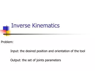
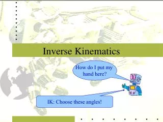
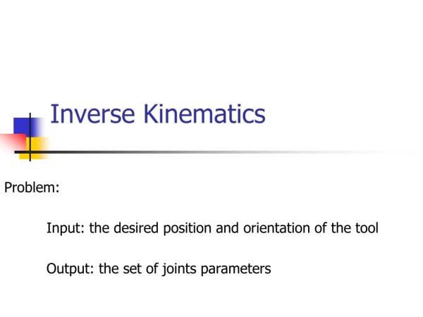
2. Inverse Kinematics • Given a desired position (P) & orientation (R) of the end-effector Find the joint variables which can bring the robot to the desired configuration.

3. A Simple Example Revolute and Prismatic Joints Combined Finding : More Specifically: (x , y) arctan2() specifies that it’s in the first quadrant Y S 1 Finding S: X

4. Solvability Given the numerical value of we attempt to find values of The PUMA 560: Given as 16 numerical values, solve for6 joint angles, 12 equations and 6 unknowns 6 equations and 6 unknowns (nonlinear, transcendental equations)

5. Inverse Kinematics • More difficult. • The equations to solve are nonlinear thus systematic closed-form solution is not always available. • Solution not unique. • Redundant robot. • Elbow-up/elbow-down configuration. • Robot dependent. 2 solutions!

6. The Workspace • Workspace: volume of space which can be reached by the end effector • Dextrous workspace: volume of space where the end effector can be arbitrarily oriented • Reachable workspace: volume of space which the robot can reach in at least one orientation

7. Two-link manipulator If l1 = l2 reachable work space is a disc of radius 2l1. The dextrous Workspace is a point: origin If l1l2 there is no dextrous workspace. The reachable work space is a ring of outer radius l1 + l2 and inner radius l1 - l2

8. Existence of Solutions • A solution to the IKP exists if the target belongs to the workspace. • Workspace computation may be hard. In practice it is made easy by special design of the robot.

9. Multiple Solutions • The IKP may have more than one solution. We need to be able to calculate all the possible solutions. • The system has to be able to choose one. 2 solutions! The closest solution: the solution which minimizes the amount that each joint is required to move.

10. The Closest Solution in Joint Space • Weights might be applied. Selection favors moving smaller joints rather than moving larger joints when a choice exist. • The presence of obstacles.

11. Two Possible Solutions In the absence of obstacles the upper configuration is selected

12. Another 4 solution Number of Solutions Depends upon the number and range of joints and also is a function of link parameters a,a,d 8 solutions exits 4 Solutions of the PUMA 560

13. Number of Solutions vs. Nonzero ai The more the link length parameters are nonzero, the bigger the maximum number of solutions!

14. Solvability • All systems with revolute and prismatic joints having total of 6 D.O.F in a single series chain are solvable. • But this general solution is a numerical one. • Robots with analytic solution: several intersecting joint axes and/or many i = 0, 90o.

15. Methods of Solutions • A manipulator is solvable if the joint variables can be determined by an algorithm. The algorithm should find all possible solutions. closed form solutions numerical solutions • Solutions

16. Numerical Solutions • Results in a numerical, iterative solution to system of equations, for example Newton/Raphson techniques. • Unknown number of operations to solve. • Only returns a single solution. • Accuracy is dictated by user. • Because of these reasons, this is much less desirable than a closed-form solution. • Can be applied to all robots.

17. Closed-form solutions Analytical solution to system of equations Can be solved in a fixed number of operations (therefore, computationally fast/known speed) Results in all possible solutions to the manipulator kinematics Often difficult or impossible to find Most desirable for real-time control Most desirable overall

18. Closed-form solutions Given a 6 axis robot. It can be proven that there exists a closed form solution for inverse kinematics: • If three adjacent revolute joint axes intersect at a point (PUMA, Stanford). • If three adjacent revolute joint axes are parallel to one another (MINIMOVER). In any case algebraic or geometric intuition is required to obtain closed form solutions.

19. Methods of Solutions In general the IK problem can be solved by various methods such as: • Inverse Transform ( Paul, 1981) • Screw Algebra (Kohli 1975) • Dual Matrices (Denavit 1956) • Iterative (Uicker 1964) • Geometric approach (Lee 1984) • Decoupling of position and orientation (Pieper 1968)

20. Closed-form Solutions We are interested in closed-form solutions: 1. Algebraic methods 2. Geometric methods

21. Algebraic solution Consider a 3-link manipulator We can derive kinematic equations:

22. i i-1 i-1 di i 1 0 0 0 1 2 0 L1 0 2 3 0 L2 0 3 Algebraic solution D-H transformation

23. Algebraic Solution

24. Algebraic Solution The kinematics of the example seen before are: Assume goal point is specified by 3 numbers:

25. Algebraic Solution By comparison, we get the four equations: Summing the square of the last 2 equations: From here we get an expression for c2 And finally:

26. Algebraic Solution • The arc cosine function does not behave well as its accuracy in determining the angle is dependant on the angle ( cos(q)=cos(-q)). • When sin(q) approaches zero, division by sin(q) give inaccurate solutions. • Therefore an arc tangent function which is more consistent is used.

27. Algebraic Solution Using c12=c1c2-s1s2 and s12= c1s2-c2s1: where k1=l1+l2c2and k2=l2s2. To solve these eqs, set r=+ k12+k22 and =Atan2(k2,k1).

28. k1 l2 k2 2  l1 Algebraic Solution Then: k1=r cos  , k2=r sin  ,and we can write: x/r= cos cos 1 - sin sin 1 y/r= cos sin 1 + sin cos 1 or: cos(+1) = x/r, sin(+1) =y/r

29. Algebraic Solution Therefore: +1 = atan2(y/r,x/r) = atan2(y,x) And so: 1 = atan2(y,x) - atan2(k2,k1) Finally, 3 can be solved from: 1+2+3 = 

30. y a2 a1 x Geometric Solution Two-link Planar Manipulator

31. Geometric Solution • Applying the “law of cosines”: • We should try to avoid using the arccos function because of inaccuracy.

32. Geometric Solution The second joint angle q2is then found accurately as: Because of the square root, two solutions result:

33. Geometric Solution q1 is determined uniquely given q2 q1=f-y Note the two different solutions for q1corresponding to the elbow-down versus elbow-up configurations

34. Examples: IK Solution for PUMA 560 Algebraic Solution for UNIMATIONPUMA 560 We wish to Solve (4.54) For qi when 06T is given as numeric values

35. Examples: IK Solution for PUMA 560 • Paul (1981) suggest pre multiplying the above matrix (4.54) by its unworn inverse transform successively and determine the unknown angle from the elements of the resultant matrix equation.

36. Examples: IK solution for PUMA 560 By multiplying both sides of (4.54) Inverting 01T we get: (4.56)

37. Examples: IK Solution for PUMA 560 • 16T from (3.13) is:

38. Examples: IK solution for PUMA 560 By adapting 16T from (3.13) and equating elements we have Using trigonometric substitution: We obtain Using difference of angles:

39. Examples: IK Solution for PUMA 560 And so: Solution for q1: Note: two possible solution for q1

40. Examples: IK Solution for PUMA 560 By equating elements (1,4) and also (3,4) from Equ. (4.56): By squaring and addition of resulting equations and Equ. (4.57): Where

41. Examples: IK Solution for PUMA 560 The above equation is only dependant on q3 so with similar procedure we get: again two different solution for q3. We may rewrite (4.54) as (4.70)

42. Examples: IK Solution for PUMA 560 By adapting 36T from (3.11) and equating (1,4) and (2,4) we have We solve for q23 as Four possible solutions for q2

43. Examples: IK Solution for PUMA 560 By equating elements (1,3) and also (3,3) from (4.70) :

44. Examples: IK Solution for PUMA 560 We continue similar procedure for rest of the Parameters…

45. Examples: IK Solution for PUMA 560 Other possible solutions : After all eight solutions have been computed, some of them may have to be discarded because of joint limitations. Usually the one closest to present manipulator configuration is chosen.

46. Pieper’s Solution When Three Axes Intersect (E.G, Spherical Wrists) • A completely general robot with six degrees of freedom does not have a closed form solution, however special cases can be solved. • The technique involves decoupling the position and orientation problems. The position problem positions the wrist center, while the orientation problem completes the desired orientation.

47. Pieper’s Solution This method applies to all six joints revolute, with the last 3 intersection It can be applied to majority of industrial robots

48. Z 5 Z d 4 6 Z P 6 c d {0} Pieper’s Solution: Basic Concept First, the location of the wrist center, pc is found from the given tool position (d) and the tool pointing direction (here z6). Since the wrist center location depends on the first three joint variables, this results in three equations and three unknowns which are solved for q1–q3. Then, the relative wrist orientation R63 which is a function of the last three joint variables, q4–q6 is found from the arm orientation R30 and the given tool orientation R60. The relative wrist orientation is set equal to the kinematic description of R63and the last 3 joint variables are solved.

49. Pieper’s SolutionStep-by-step Procedure • Start with the given tool pose, as . • Solve portions of the forward kinematics to find find . • Find the location of the wrist center, as (last column of ) - (tool offset length) x (thirdcolumn of ). • Set = last column of and solve for for . • Solve as (put into ). • Set equal to and solve for . • Along the way, keep track of the number of solutions for each joint variable.

50. {W} {B} {T} {G} {S} Standard Frames