Download
1 / 48
500 likes | 765 Vues
Chapter 3 Solving Problems by Searching. Search. Search permeates all of AI An intelligent agent is trying to find a set or sequence of actions to achieve a goal. What choices are we searching through? Problem solving Action combinations (move 1, then move 3, then move 2...)

E N D
Search • Search permeates all of AI • An intelligent agent is trying to find a set or sequence of actions to achieve a goal. • What choices are we searching through? • Problem solvingAction combinations (move 1, then move 3, then move 2...) • Natural language Ways to map words to parts of speech • Computer vision Ways to map features to object model • Machine learning Possible concepts that fit examples seen so far • Motion planning Sequence of moves to reach goal destination • This is a goal-based agent
3.1 Problem-solving Agent Process flow: SimpleProblemSolvingAgent(percept) state = UpdateState(state, percept) if sequence is empty then goal = FormulateGoal(state) problem = FormulateProblem(state, g) sequence = Search(problem) action = First(sequence) sequence = Rest(sequence) Return action
Assumptions Environment is static Static or dynamic?
Assumptions Environment is fully observable Static or dynamic? Fully or partially observable?
Assumptions Environment is discrete Static or dynamic? Fully or partially observable? Discrete or continuous?
Assumptions Environment is deterministic Static or dynamic? Fully or partially observable? Discrete or continuous? Deterministic or stochastic?
Assumptions Environment is sequential Static or dynamic? Fully or partially observable? Discrete or continuous? Deterministic or stochastic? Episodic or sequential?
Assumptions Static or dynamic? Fully or partially observable? Discrete or continuous? Deterministic or stochastic? Episodic or sequential? Single agent or multiple agent?
Assumptions Static or dynamic? Fully or partially observable? Discrete or continuous? Deterministic or stochastic? Episodic or sequential? Single agent or multiple agent?
3.2 Search Example Formulate goal: Be in Bucharest. Formulate problem: states are cities, operators drive between pairs of cities Find solution: Find a sequence of cities (e.g., Arad, Sibiu, Fagaras, Bucharest) that leads from the current state to a state meeting the goal condition
Search Space Definitions • State • A description of a possible state of the world • Includes all features of the world that are pertinent to the problem • Initial state • Description of all pertinent aspects of the state in which the agent starts the search • Goal test • Conditions the agent is trying to meet • Goal state • Any state which meets the goal condition • Action • Function that maps (transitions) from one state to another
Search Space Definitions • Problem formulation • Describe a general problem as a search problem • Solution • Sequence of actions that transitions the world from the initial state to a goal state • Solution cost (additive) • Sum of the cost of operators • Alternative: sum of distances, number of steps, etc. • Search • Process of looking for a solution • Search algorithm takes problem as input and returns solution • We are searching through a space of possible states • Execution • Process of executing sequence of actions (solution)
Problem Formulation A search problem is defined by the Initial state (e.g., Arad) Operators (e.g., Arad -> Zerind, Arad -> Sibiu, etc.) Goal test (e.g., at Bucharest) Solution cost (e.g., path cost)
3.2.1 Example Problems – Eight Puzzle States: tile locations Initial state: one specific tile configuration Operators: move blank tile left, right, up, or down Goal: tiles are numbered from one to eight around the square Path cost: cost of 1 per move (solution cost same as number of most or path length) Eight Puzzle http://mypuzzle.org/sliding
Example Problems – Robot Assembly • States: real-valued coordinates of • robot joint angles • parts of the object to be assembled • Operators: rotation of joint angles • Goal test: complete assembly • Path cost: time to complete assembly
Example Problems – Towers of Hanoi • States: combinations of poles and disks • Operators: move disk x from pole y to pole z subject to constraints • cannot move disk on top of smaller disk • cannot move disk if other disks on top • Goal test: disks from largest (at bottom) to smallest on goal pole • Path cost: 1 per move Towers of Hanoi: http://www.mathsisfun.com/games/towerofhanoi.html
Example Problems – Rubik’s Cube States: list of colors for each cell on each face Initial state: one specific cube configuration Operators: rotate row x or column y on face z direction a Goal: configuration has only one color on each face Path cost: 1 per move
Example Problems – Eight Queens States: locations of 8 queens on chess board Initial state: one specific queens configuration Operators: move queen x to row y and column z Goal: no queen can attack another (cannot be in same row, column, or diagonal) Path cost: 0 per move Eight queens: http://www.coolmath-games.com/Logic-eightqueens/index.html
Example Problems – Missionaries and Cannibals • States: number of missionaries, cannibals, and boat on near river bank • Initial state: all objects on near river bank • Operators: move boat with x missionaries and y cannibals to other side of river • no more cannibals than missionaries on either river bank or in boat • boat holds at most m occupants • Goal: all objects on far river bank • Path cost: 1 per river crossing Missionaries and cannibals: http://www.plastelina.net/game2.html
Example Problems –Water Jug • States: Contents of 4-gallon jug and 3-gallon jug • Initial state: (0,0) • Operators: • fill jug x from faucet • pour contents of jug x in jug y until y full • dump contents of jug x down drain • Goal: (2,n) • Path cost: 1 per fill
3.2.2 Real-world Problems Graph coloring Protein folding Game playing Airline travel Proving algebraic equalities Robot motion planning
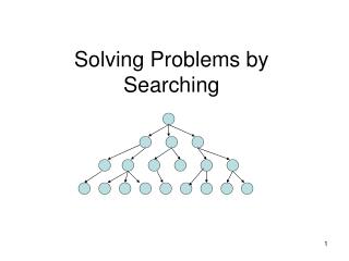
3.3 Searching for SolutionsVisualize Search Space as a Tree States are nodes Actions are edges Initial state is root Solution is path from root to goal node Edges sometimes have associated costs States resulting from operator are children
Search Problem Example (as a tree)(start: Arad, goal: Bucharest.)
3.4 Uninformed Search Strategies Uninformed search (also called blind search): search strategies that have no additional information about states beyond that provided in problem definition. All they can do is generate successors and distinguish a goal from a non-goal state. Open = initial state // open list is all generated states // that have not been “expanded” While open not empty // one iteration of search algorithm state = First(open) // current state is first state in open Pop(open) // remove new current state from open if Goal(state) // test current state for goal condition return “succeed” // search is complete // else expand the current state by // generating children and // reorder open list per search strategy else open = QueueFunction(open, Expand(state)) Return “fail”
Search Strategies • Search strategies differ only in QueuingFunction: FIFO queue, LIFO queue (known as a stack), priority queue. • Features by which to compare search strategies • Completeness (always find solution) • Cost of search (time and space) • Cost of solution, optimal solution • Make use of knowledge of the domain • “uninformed search” vs. “informed search”
3.4.1 Breadth-First Search breadth-first searching expands a node and checks each of its successors for a goal state before expanding any of the original node's successors (unlike depth-first search).
Breadth-First Search Generate children of a state, QueueingFn adds the children to the end of the open list Level-by-level search Order in which children are inserted on open list is arbitrary In tree, assume children are considered left-to-right unless specified differently Number of children is “branching factor” b
Analysis • Assume goal node at level d with constant branching factor b • Time complexity (measured in #nodes generated) • 1 (1st level ) + b (2nd level) + b2 (3rd level) + … + bd (goal level) + (bd+1 – b) = O(bd) • This assumes goal on far right of level • Space complexity • complexity : O(bd) • Exponential time and space • Features • Simple to implement • Complete • Finds shortest solution (not necessarily least-cost unless all operators have equal cost)
Analysis • See what happens with b=10 • expand 10,000 nodes/second • 1,000 bytes/node
3.4.3 Depth-First Search Depth-first is an unintelligent algorithm (i.e., no heuristic is used) which starts at an initial state and proceeds as follows: • Check if current node is a goal state. • If not, expand the node, choose a successor of the node, and repeat. • If a node is a terminal state (but not a goal state), or all successors of a node have been checked, return to that node’s parent and try another successor.
3.4.3 Depth-First Search • QueueingFn adds the children to the front of the open list • BFS emulates FIFO queue • DFS emulates LIFO stack • Net effect • Follow leftmost path to bottom, then backtrack • Expand deepest node first
DFS Examples Example trees
Analysis • Time complexity • In the worst case, search entire space • Goal may be at level d but tree may continue to level m, m>=d • O(bm) • Particularly bad if tree is infinitely deep • Space complexity • Only need to save one set of children at each level • 1 + b + b + … + b (m levels total) = O(bm) • For previous example, DFS requires 118kb instead of 10 petabytes for d=12 (10 billion times less) • Benefits • Solution is not necessarily shortest or least cost • If many solutions, may find one quickly (quickly moves to depth d) • Simple to implement • Space often bigger constraint, so more usable than BFS for large problems
Avoiding Repeated States Can we do it? Do not return to parent or grandparent state Do not create solution paths with cycles Do not generate repeated states (need to store and check potentially large number of states)
3.4.2 Uniform Cost Search (Branch&Bound) • QueueingFn is SortByCostSoFar • Cost from root to current node n is g(n) • Add operator costs along path • First goal found is least-cost solution • Space & time can be exponential because large subtrees with inexpensive steps may be explored before useful paths with costly steps • If costs are equal, time and space are O(bd) • Otherwise, complexity related to cost of optimal solution
UCS Example Uniform cost searches always expand the node with the lowest total path cost from the initial node. Thus, they are always optimal (since any cheaper solution would already have been found.) Their salient characteristic is the fact that they start from the initial start node when they calculate the path cost in the search.
Comparison of Search Techniques C*: the cost of the optimal solution ε: every action cost at least ε
3.4.5 Iterative Deepening Search The iterative deepening search combines the positive elements of breadth-first and depth-first searching to create an algorithm which is often an improvement over each method individually. A node at the limit level of depth is treated as terminal, even if it would ordinarily have successor nodes. If a search "fails," then the limit level is increased by one and the process repeats. The value for the maximum depth is initially set at 0 (i.e., only the initial node).
Iterative Deepening Search • DFS with depth bound • QueuingFn is enqueue at front as with DFS • Expand(state) only returns children such that depth(child) <= threshold • This prevents search from going down infinite path • First threshold is 1 • If do not find solution, increment threshold and repeat
Analysis • Time complexity (number of generated nodes) • N(IDS) = (d)b + (d-1) b2 + … + (1) bd (d: depth) • O(bd) • Search Space O(bd)
Analysis • Repeated work is approximately 1/b of total work • Example: b=10, d=5 • N(BFS) = 1,111,100 • N(IDS) = 123,450 • Features • Shortest solution, not necessarily least cost • Is there a better way to decide threshold?
Comparison of Search Techniques C*: the cost of the optimal solution ε: every action cost at least ε
3.4.6 Bidirectional Search • Search forward from initial state to goal AND backward from goal state to initial state • Can prune many options • Considerations • Which goal state(s) to use • How determine when searches overlap • Which search to use for each direction • Here, two BFS searches • Time and space is O(bd/2)