Download

1 / 38
380 likes | 401 Vues
Learn about inverse problems, how to approach them, and gain insights from them through the example of Johnny and Susie's monthly earnings. Explore contour plots, uncertainties, and the power of Chi-square analysis.

E N D
Inverse Problems: What are they, how can we approach them, and what can we learn from them?
Johnny works two jobs. This past April he made $2100 at the first, and an additional $1300 at the second. How much did Johnny make in total for the month of April? Consider the Following:
Johnny works two jobs. This past April he made $2100 at the first, and an additional $1300 at the second. How much did Johnny make in total for the month of April? Consider the Following: Not surprisingly, Johnny has made $3400 for April.
Susie also works two jobs. If Susie made $4500 for herself during the month of April, how much did she earn at each job individually? But How About This:
Susie also works two jobs. If Susie made $4500 for herself during the month of April, how much did she earn at each job individually? But How About This: There isn't a single answer for this question!
Here's a general diagram of the situations we just had.
Job #1 Salary Total Income Job #2 Salary In Johnny's case, we combined A & B to get C.
Job #1 Salary Total Income Job #2 Salary But in Susie's case, we only had C to try finding A & B.
? Job #1 Salary Total Income ? Job #2 Salary This is an example of an inverse problem; how can we attempt to solve it?
One way is by utilizing contours, like on this map of Hawaii.
Note that the contours represent lines of constant elevation.
We'll use that same idea, but applied in a different way.
For example, here's the combination A+B, where we require that C = 75.
All points on the blue contour represent A+B = 75.
Here, the line in red represents the requirement that A+B = 110.
We could combine A & B any way we want actually; here are contours for A•B.
So, in the regular problem, we find a unique answer C from our combined parameters A & B. • However, in the inverse problem, we find a contour of solutions for A & B from a specified value for C. • Mathematically speaking, there are infinitely-many solutions!
Things start to get even more complex when we take uncertainties into account.
This is a Normal Curve, also called a Bell Curve. Data can often be represented by this type of graph.
Center Spread Notice how the graph has both a center (or mean) & a spread (or standard deviation.)
The numbers at the bottom are a measure of how far from the center a value is: greater means farther away, and thus more unlikely to occur.
We can look at the value of Chi-square for C at many locations on our contour plot.
The higher the value, the less likely that combination of A & B is (given our requirements on C.)
Suppose we are interested in the combination: A + B = C Say we also know that C = 110, with an uncertainty of 10. We might guess that we'd get a simple contour of possible A & B combos, like before. Is that the case?... Let's Try it Out:
The darker regions are more likely combos for A & B, while lighter regions are more unlikely.
See how the uncertainty in C has spread out the combinations of A & B from a single contour?
As we can see, there are a LOT of reasonable possibilities for A & B in this situation.
Say we were also interested in the combination: A – B = D Suppose we know that D = 30, with an uncertainty of 5. We realize now that we'll get a swath, just like with C from before. But what will it look like?... Consider, Though:
By itself, this isn't really any more interesting. If we put both regions together, though...
...Presto! We've shrunk the possible A & B combinations dramatically.
In such situations, this Chi-square analysis has the potential to be quite powerful.
Relationship: Parameters {A,B} & Constraint C {A,B} → C: Unique (Normal Problem) C → {A,B}: Contour (Inverse Problem) Uncertainties on C: Contour morphs into Region Compile C with D: Regioncan shrink smaller Apply this idea to tackle real problems! In Summary: