Optically polarized atoms
620 likes | 880 Vues
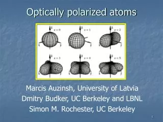
Optically polarized atoms. Marcis Auzinsh, University of Latvia Dmitry Budker, UC Berkeley and LBNL Simon M. Rochester, UC Berkeley. Chapter 5: Atomic transitions. Preliminaries and definitions Transition amplitude Transition probability Analysis of a two-level problem. See also:.

Optically polarized atoms
E N D
Presentation Transcript
Optically polarized atoms Marcis Auzinsh, University of Latvia Dmitry Budker, UC Berkeley and LBNL Simon M. Rochester, UC Berkeley
Chapter 5: Atomic transitions • Preliminaries and definitions • Transition amplitude • Transition probability • Analysis of a two-level problem See also: Problem 3.1 http://socrates.berkeley.edu/~budker/Tutorials/
Periodic perturbation Two-level system Initial Condition:
Solving the problem… • There are many ways to solve for the probability of finding the system in either of the two states, including • Solve time-dependent Schrödinger equation • Make a unitary transformation to get rid of time dependence of the perturbation (this is equivalent to going into “rotating frame”) • Solve the Liouville equation for the density matrix • We will discuss all this in due time, but let us skip to the results for now…
P – probability of finding system in the upper state • Maximal-amplitude sinusoidal oscillations • P=sin2(V0t)=[1-cos (ΩRt)]/2 ; ΩR=2V0 - Rabi frequency • At small t P t 2 an interference effect (amplitudes from different dtadd) • Stimulated emission and stimulated absorption
P – probability of finding system in the upper state • Non-maximal-amplitude sinusoidal oscillations • Oscillation frequency: |Δ| • For the cases where always P(t)<<1 :
Including the effect of relaxation • Decay to unobserved levels (outside the system) • Damped oscillations
Including the effect of relaxation • Overdamped regime – no oscillations • This occurs for Γ>2ΩR • The system behaves as if there is no relaxation for small t • General analytical formula :
Selection rules • Certain quantities must remain conserved in a transition • An easy way to think about it is the photon picture • Conserved quantities: energy, momentum, total angular momentum, … • We have many angular momenta for atoms: L S J I F • Forget I J=F for now (to make life easier) • For electric-dipole (E1) transitions, Jphot= Sphot=1; Lphot=0 • Adding or subtracting angular momentum one changes angular momentum of a system by 0,+1, or -1 • Also, 00 transitions are forbidden • Generally, we have triangle rule
Entertaining Interlude: cutting a stickor getting to know the triangle rule A stick is randomly cut into three Q. What is the probability that one can make a triangle out of the resultant sticks ? A. 1/4
Another form of the • 00 transitions are forbidden rule Selection rules Q: What changes when J changes, L, S, or both ? • A:it is L that changes orbital rearrangement • In classical electrodynamics, emission and absorption have to do with accelerating charges • Additional selection rules (good to the extent L,S are good quantum #s):
Parity of atomic states • Spatial inversion (P) : • Or, in polar coordinates:
Parity of atomic states • It might seem that P is an operation that may be reduced to rotations • This is NOTthe case • Let’s see what happens if we invert a coordinate frame : • Now apply a rotation around z’ Right-handed frame left handed • P does NOTreduce to rotations !
Parity of atomic states • An amazing fact : atomic Hamiltonian is rotationally invariant but is NOT P-invariant • We will discuss parity nonconservation effects in detail later on in the course…
This is because: Parity of atomic states • In hydrogen, the electron is in centro-symmetric nuclear potential • In more complex atoms, an electron sees a more complicated potential • If we approximate the potential from nucleus and other electrons as centro-symmetric (and not parity violating) , then : Wavefunctions in this form are automatically of certain parity : • Since multi-electron wavefunction is a (properly antisymmetrized) product of wavefunctions for each electron, parity of a multi-electron state is a product of parities for each electron:
Comments on multi-electron atoms • Potential for individual electrons is NOT centrosymmetric • Angular momenta and parity of individual electrons are not exact notions (configuration mixing, etc.) • But for the system of all electrons, total angular momentum and parity are good ! • Parity of a multi-electron state: W A R N I N G
Parity of atomic states A bit of formal treatment… • Hamiltonian is P-invariant (ignoring PNC) : P-1HP=H • spatial-inversion operator commutes with Hamiltonian : [P,H]=0 • stationary states are simultaneous eigenstates of H and P • What about eigenvalues (p; Pψ=pψ) ? • Note that doing spatial inversion twice brings us back to where we started • P2 ψ=P(P ψ)=P(pψ)=p(Pψ)=p2 ψ. This has to equal ψ p2=1 p=1 • p=1 – even parity; p=-1 – odd parity
Back to dipole transitions • Transition amplitude : < ψ2|d|ψ1> , where d=er is the dipole operator • For multi-electron atoms dipole operator is sum over electrons : d=Sidi • However, the operator changes at most one electron at a time, so for pure configurations, transitions are only allowed between states different just by one electron, for example (in Sm) : (Xe)4f66s6p (Xe)4f66s7s (Xe)4f66s6p (Xe)4f67p6p (Xe)4f66s6p (Xe)4f67p7s
Parity selection rule • Transition amplitude: Odd under P • This means that for the amplitude not to vanish, the product must also be P-odd • Initial and final states must be of opposite parity
Higher-multipole radiative transitions • If electric-dipole-transition (E1) selection rules not satisfied forbidden transitions • E1 are due to the electric-dipole Hamiltonian: Hd=-dE • In analogy, there are magnetic-dipole transitions due to: Hm=-μB • Also, there are electric-quadrupole transitions due to: • Each type of transitions has associated selection rules
Magnetic-dipole transitions • Let us estimate the ratio of the transition matrix elements for M1 and E1 • A typical atomic electric-dipole moment is ea • A typical atomic magnetic-dipole moment is μ0 • Transition probability (assuming same wavelength):
m r P-odd P-odd i P-even ! Magnetic-dipole transitions • What are the M1 selection rules ? • Imagine a transition between levels for which E1 angular-momentum selection rules are satisfied, but parity rule is not • Notice: mis a pseudo-vector (= axial vector), i.e. it is invariant with respect to spatial inversion. Imagine a current loop: M1 transitions occur between states of same parity
Magnetic-dipole transitions Important M1 transitions occur : • between Zeeman sublevels of the same state: NMR, optical-pumping magnetometers, etc. • between hyperfine-structure levels: atomic clocks, the 21-cm line This horn antenna, now displayed in front of the Jansky Lab at NRAO in Green Bank, WV, was used by Harold Ewen and Edward Purcell, then at the Lyman Laboratory of Harvard University, in the first detection of the 21 cm emission from neutral hydrogen in the Milky Way. The emission was first detected on March 25, 1951. See: http://www.nrao.edu/whatisra/hist_ewenpurcell.shtml
Some other multipole transitions Electric-quadrupole (E2) transitions No parity change ! With LS coupling, we also have This can be continued (E3,M2,…)
How to calculate E1 transition probability • In quantum mechanics: transition probability between the initial and final state is proportional to:
How to calculate E1 transition probability • Let us recall how this comes about… • For single-electron atom, neglecting nuclear spin • Can this be simplified ? • Let’s relate the light electric field and the vector potential • We can relate electron momentum to atomic electric field; this shows that if the light field is much weaker than the atomic field, the term quadratic in A can be neglected; this is usually the case (except modern ultra-short laser pulses)
0 How to calculate E1 transition probability • In this approximation and neglecting electron spin :
Only annihilation operator contributes How to calculate E1 transition probability • To calculate transition probability, take matrix elements of perturbation between combined states of light and atoms: • For absorption, n+1n • Here we used essential results from QED: • These reflect the essential bosonic properties of light, and relate stimulated emission and absorption with spont. em. +1
How to calculate E1 transition probability • Next, we apply the Dipole Approximation : • and make use of the Heisenberg eqn:
Interlude: the Heisenberg Eqn. • Classical momentum: • In QM, time derivative of any operator is given by commutator with the Hamiltonian
How to calculate E1 transition probability • With this we have : • We see that for absorption, amplitude is • while for emission, amplitude is • Scalar product of vectors can be written as
“3j symbol” How to calculate E1 transition probability • With this we have : • We next concentrate on the ME of the components of the dipole moment • The dynamic and angular parts are separated using the all-important Wigner-Eckart Theorem
Reduced matrix element “3j symbol” • Wigner-Eckart Theorem • Useful property : How to calculate E1 transition probability Actually, with common phase conventions, ||d|| are real !
Represent the geometric part of transition amplitude • Reduced matrix element – no reference to projections: dynamic part • 3j symbols are standard functions in MathematicaTM • Contain selection rules for angular-momenta addition, including the triangular condition • and the projection rule 3j symbols
Interlude: why is M=0M’=0 transition forbidden for J=J’=1 ? • J=1, J’=1, photon – vector “particles” • Duality between q (or M) and polarization vector • Building final vector out of initial polarization vectors: • =0 when both vectors are along z The only possibility:
“6j symbol” Reduced matrix elements in LS coupling • As far as LS coupling holds, we can make further simplifications; label states conspicuously : • Only L changes in E1 transitions • Note: no mention of projections • 6j symbols obey a number of triangular conditions
Triangular conditions for 6j symbols • Each of the following angular momenta must form a triangle: • 6j symbols are real numbers • 6j symbols are standard functions in MathematicaTM • Our discussion translates to hyperfine transitions with LJ, L’J’ , JF, J’F’,S=S’I
2P3/2 2P1/2 D1 D2 2S1/2 Example: alkali D lines • Compare transition strengths : • Evaluate : • D2 is twice stronger than D1
2P3/2 2P1/2 D1 D2 2S1/2 Example: alkali D lines • Reduced matrix elements can be extracted from lifetimes: • Prediction (D2 is twice stronger than D1) confirmed by experiment:
D2 D1 Hyperfine structure • Line strength : • Examples: alkali atoms with I=3/2 (7Li, 23Na, 39K, 41K, 87Rb)
Hyperfine structure • Normalization: • To compare line strengths for different manifolds, need to account for the difference in reduced ME • Combining formulae for fine and hyperfine structure:
Multipole transitions forSegwayTM riders • As opposed to pedestrians • In the E1 approximation, we neglect spatial variation of light field over the size of an atom and set • This is because: • Another approximation we made was to neglect coupling of light B-field with electron’s magnetic moment μ. Including this, we have • Coulomb-gauge Hamiltonian:
Multipole transitions forSegwayTM riders • Expanding the exponent: • It is possible to build a classification of multipole transitions based on this expansion, for example, E2 first appears in the second term • However, complications: magnetic multipoles, etc. • Nice way to sort this out: photon picture: • Multipolarity determined by j : • E or M ? Photon Quantum Numbers
Spherical Bessel Functions Legendre Polynomials Multipole transitions for SegwayTM ridersconnecting the photon and semiclassical pictures • The Rayleigh’s formula: • Property of Bessel functions: expanding we get nonzero terms with
Multipole transitions for SegwayTM riderssome examples • E1: j=1 (dipole); l=0 or 2(because j=l1) For l=0, nonzero terms in the Rayleigh’s formula are 1, (kr)2, … • E2: j=2 (quadrupole); l=1 or 3(because j=l1) For l=1, nonzero terms in Rayleigh’s formula are (kr), (kr)3, … For l=3, nonzero terms in Rayleigh’s formula are (kr)3, (kr)5, … • M1: j=1 (dipole); l=1(because j=l) For l=1, nonzero terms in Rayleigh’s formula are (kr), (kr)3, … • The photon picture is consistent with semiclassical one