Classification: Definition

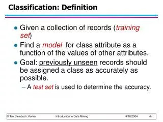
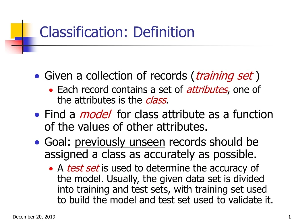
Classification: Definition • Given a collection of records (training set ) • Each record contains a set of attributes, one of the attributes is the class. • Find a model for class attribute as a function of the values of other attributes. • Goal: previously unseen records should be assigned a class as accurately as possible. • A test set is used to determine the accuracy of the model. Usually, the given data set is divided into training and test sets, with training set used to build the model and test set used to validate it.

Training Data Classifier (Model) Classification Process (1): Model Construction Classification Algorithms IF rank = ‘professor’ OR years > 6 THEN tenured = ‘yes’

Classifier Testing Data Unseen Data Classification Process (2): Use the Model in Prediction (Jeff, Professor, 4) Tenured?

Classification by Decision Tree Induction • Decision tree • A flow-chart-like tree structure • Internal node denotes a test on an attribute • Branch represents an outcome of the test • Leaf nodes represent class labels or class distribution • Decision tree generation consists of two phases • Tree construction • At start, all the training examples are at the root • Partition examples recursively based on selected attributes • Tree pruning • Identify and remove branches that reflect noise or outliers • Use of decision tree: Classifying an unknown sample • Test the attribute values of the sample against the decision tree

categorical categorical continuous class Example of a Decision Tree Splitting Attributes Refund Yes No NO MarSt Married Single, Divorced TaxInc NO < 80K > 80K YES NO Model: Decision Tree Training Data

NO Another Example of Decision Tree categorical categorical continuous class Single, Divorced MarSt Married NO Refund No Yes TaxInc < 80K > 80K YES NO There could be more than one tree that fits the same data!

Refund Yes No NO MarSt Married Single, Divorced TaxInc NO < 80K > 80K YES NO Apply Model to Test Data Test Data Start from the root of tree.

Refund Yes No NO MarSt Married Single, Divorced TaxInc NO < 80K > 80K YES NO Apply Model to Test Data Test Data

Apply Model to Test Data Test Data Refund Yes No NO MarSt Married Single, Divorced TaxInc NO < 80K > 80K YES NO

Apply Model to Test Data Test Data Refund Yes No NO MarSt Assign Cheat to “No” Married Single, Divorced TaxInc NO < 80K > 80K YES NO

Algorithm for Decision Tree Induction • Basic algorithm (a greedy algorithm) • Tree is constructed in a top-down recursive divide-and-conquer manner • At start, all the training examples are at the root • Attributes are categorical (if continuous-valued, they are discretized in advance) • Examples are partitioned recursively based on selected attributes • Test attributes are selected on the basis of a heuristic or statistical measure (e.g., information gain) • Conditions for stopping partitioning • All samples for a given node belong to the same class • There are no remaining attributes for further partitioning – majority voting is employed for classifying the leaf • There are no samples left

General Structure of Hunt’s Algorithm • Let Dt be the set of training records that reach a node t • General Procedure: • If Dt contains records that belong the same class yt, then t is a leaf node labeled as yt • If Dt is an empty set, then t is a leaf node labeled by the default class, yd • If Dt contains records that belong to more than one class, use an attribute test to split the data into smaller subsets. Recursively apply the procedure to each subset. Dt ?

Refund Refund Yes No Yes No Don’t Cheat Marital Status Don’t Cheat Marital Status Single, Divorced Refund Married Married Single, Divorced Yes No Don’t Cheat Taxable Income Cheat Don’t Cheat Don’t Cheat Don’t Cheat < 80K >= 80K Don’t Cheat Cheat Hunt’s Algorithm Don’t Cheat

Tree Induction • Greedy strategy. • Split the records based on an attribute test that optimizes certain criterion. • Issues • Determine how to split the records • How to specify the attribute test condition? • How to determine the best split? • Determine when to stop splitting

How to Specify Test Condition? • Depends on attribute types • Nominal • Ordinal • Continuous • Depends on number of ways to split • 2-way split • Multi-way split

CarType Family Luxury Sports CarType {Sports, Luxury} {Family} Splitting Based on Nominal Attributes • Multi-way split: Use as many partitions as distinct values. • Binary split: Divides values into two subsets. Need to find optimal partitioning.

Splitting Based on Continuous Attributes • Different ways of handling • Discretization to form an ordinal categorical attribute • Static – discretize once at the beginning • Dynamic – ranges can be found by equal interval bucketing, equal frequency bucketing (percentiles), or clustering. • Binary Decision: (A < v) or (A  v) • consider all possible splits and finds the best cut • can be more compute intensive

Splitting Based on Continuous Attributes

Information Gain (ID3/C4.5) • Select the attribute with the highest information gain • Assume there are two classes, P and N • Let the set of examples S contain p elements of class P and n elements of class N • The amount of information, needed to decide if an arbitrary example in S belongs to P or N is defined as

Class C(cheat contains 3 tuples) Class NC contains 7 tuples I(C,NC) = -3/10*log(3/10) -7/10*log(7/10) = .2653 Check attribute Refund: Yes value contains 3 NC and 0 C. No value contains 4 NC and 3 C For Yes: 3/3*log3/3 +0/3log0 = 0 For No: 4/7*log(7/4)+3/7*log(7/3) = .2966 E(Refund) = 3/10*0 + 7/10*.2966= .2076 Gain= I(C,NC) - E(Refund)= .0577 Refund attribute Information Gain Don’t Cheat

Check attribute MS: Single value contains 3 NC and 3 C. Married value contains 4 NC and 0 C For Single: 3/6*log6/3 + 3/6log6/3 = .30 For Married: 4/4*log(4/4)+0/4*log(0) = 0 E(Refund) = 6/10*.3 + 4/10*.0=.18 . Gain= I(C,NC) - E(MS)= .0853 Marital Status Information Gain Don’t Cheat

Suppose that taxable income is discretized into: (0, 75], (75,100],(100, 1000000] First segment contains 3NC 0C Second segment contains 1NC 3C Third segment contains 3NC 0C For 1st segment: 3/3*log1 + 0/3*log1 = 0 For 2d segment: 1/4*log(4/1)+3/4*log(4/3) = .2442 For 3d segment we also obtain 0 E(TI) = 3/10*0 + 4/10*.2442+ 3/10*0 =.0977 Gain= I(C,NC) - E(MS)= .1676 Taxable income(TI) Information Gain Don’t Cheat

Information Gain in Decision Tree Induction • Assume that using attribute A a set S will be partitioned into sets {S1, S2 , …, Sv} • If Si contains piexamples of P and ni examples of N, the entropy, or the expected information needed to classify objects in all subtrees Si is • The encoding information that would be gained by branching on A

RID Age Income Student Credit Class: buysComputer

Class P: buys_computer = “yes” Class N: buys_computer = “no” I(p, n) = I(9, 5) =0.940 Compute the entropy for age: Hence Similarly Attribute Selection by Information Gain Computation

Extracting Classification Rules from Trees • Represent the knowledge in the form of IF-THEN rules • One rule is created for each path from the root to a leaf • Each attribute-value pair along a path forms a conjunction • The leaf node holds the class prediction • Rules are easier for humans to understand • Example IF age = “<=30” AND student = “no” THEN buys_computer = “no” IF age = “<=30” AND student = “yes” THEN buys_computer = “yes” IF age = “31…40” THEN buys_computer = “yes” IF age = “>40” AND credit_rating = “excellent” THEN buys_computer = “yes” IF age = “>40” AND credit_rating = “fair” THEN buys_computer = “no”

Stopping Criteria for Tree Induction • Stop expanding a node when all the records belong to the same class • Stop expanding a node when all the records have similar attribute values • Early termination (to be discussed later)

Table to be classified

Decision Tree Based Classification • Advantages: • Inexpensive to construct • Extremely fast at classifying unknown records • Easy to interpret for small-sized trees • Accuracy is comparable to other classification techniques for many simple data sets

Practical Issues of Classification • Underfitting and Overfitting • Missing Values • Costs of Classification

Underfitting and Overfitting (Example) 500 circular and 500 triangular data points. Circular points: 0.5  sqrt(x12+x22)  1 Triangular points: sqrt(x12+x22) > 0.5 or sqrt(x12+x22) < 1

Underfitting and Overfitting Overfitting Underfitting: when model is too simple, both training and test errors are large

Overfitting due to Noise Decision boundary is distorted by noise point

Overfitting due to Insufficient Examples Lack of data points in the lower half of the diagram makes it difficult to predict correctly the class labels of that region - Insufficient number of training records in the region causes the decision tree to predict the test examples using other training records that are irrelevant to the classification task

Notes on Overfitting • Overfitting results in decision trees that are more complex than necessary • Training error no longer provides a good estimate of how well the tree will perform on previously unseen records • Need new ways for estimating errors

Minimum Description Length (MDL) • Cost(Model,Data) = Cost(Data|Model) + Cost(Model) • Cost is the number of bits needed for encoding. • Search for the least costly model. • Cost(Data|Model) encodes the misclassification errors. • Cost(Model) uses node encoding (number of children) plus splitting condition encoding.

Metrics for Performance Evaluation • Focus on the predictive capability of a model • Rather than how fast it takes to classify or build models, scalability, etc. • Confusion Matrix: a: TP (true positive) b: FN (false negative) c: FP (false positive) d: TN (true negative)

Metrics for Performance Evaluation… • Most widely-used metric:

Limitation of Accuracy • Consider a 2-class problem • Number of Class 0 examples = 9990 • Number of Class 1 examples = 10 • If model predicts everything to be class 0, accuracy is 9990/10000 = 99.9 % • Accuracy is misleading because model does not detect any class 1 example

Cost Matrix C(i|j): Cost of misclassifying class j example as class i

Computing Cost of Classification Accuracy = 80% Cost = 3910 Accuracy = 90% Cost = 4255

Accuracy is proportional to cost if1. C(Yes|No)=C(No|Yes) = q 2. C(Yes|Yes)=C(No|No) = p N = a + b + c + d Accuracy = (a + d)/N Cost = p (a + d) + q (b + c) = p (a + d) + q (N – a – d) = q N – (q – p)(a + d) = N [q – (q-p)  Accuracy] Cost vs Accuracy

Bayesian Classification: Why? • Probabilistic learning: Calculate explicit probabilities for hypothesis, among the most practical approaches to certain types of learning problems • Incremental: Each training example can incrementally increase/decrease the probability that a hypothesis is correct. Prior knowledge can be combined with observed data. • Probabilistic prediction: Predict multiple hypotheses, weighted by their probabilities • Standard: Even when Bayesian methods are computationally intractable, they can provide a standard of optimal decision making against which other methods can be measured

Estimating a-posteriori probabilities • Bayes theorem: P(C|X) = P(X|C)·P(C) / P(X) • P(X) is constant for all classes • P(C) = relative freq of class C samples • C such that P(C|X) is maximum = C such that P(X|C)·P(C) is maximum • Problem: computing P(X|C) is unfeasible!

Naïve Bayesian Classification • Naïve assumption: attribute independence P(x1,…,xk|C) = P(x1|C)·…·P(xk|C) • If i-th attribute is categorical:P(xi|C) is estimated as the relative freq of samples having value xi as i-th attribute in class C • Computationally easy in both cases

Classification: Definition