Download
1 / 39
390 likes | 500 Vues
This document explores advanced algorithms in artificial intelligence for game playing, focusing on Alpha-Beta pruning and meta-reasoning techniques. It discusses the complexity of decision-making in games like Chess, Checkers, and Go while integrating elements of chance, such as in Backgammon. Through iterative deepening, utility computation, and machine learning, systems like IBM's Deep Blue are analyzed for their search strategies and performance. The intricate balance between legal moves and computational efficiency is examined, providing insights into optimal game strategies for AI.

E N D
double AlphaBeta(state, depth, alpha, beta) begin if depth <= 0 then return evaluation(state) //op pov for each action “a” possible from state nextstate = performAction(a, state) rval = -AlphaBeta(nextstate, depth-1, -beta, -alpha); if (rval >= beta)return rval; if (rval > alpha) alpha = rval; endfor return alpha; end
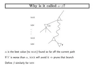
Meta-Reasoning for Search • problem: one legal move only (or one clear favourite) alpha-beta search will still generate (possibly large) search tree • similar symmetrical situations • idea: compute utility of expanding a node before expanding it • meta-reasoning (reasoning about reasoning): reason about how to spend computing time
Deep Blue • algorithm: • iterative-deepening alpha-beta search, transposition table, databases incl. openings, grandmaster games (700000), endgames (all with 5 pieces, many with 6) • hardware: • 30 IBM RS/6000 processors • software search: at high level • 480 custom chess processors for • hardware search: search deep in the tree, move generation and ordering, position evaluation (8000 features) • average performance: • 126 million nodes/sec., 30 billion position/move generated, search depth: 14 (but up to 40 plies)
Samuel’s Checkers Program (1952) • learn an evaluation function by self-play(see: machine learning) • beat its creator after several days of self-play • hardware: IBM 704 • 10kHz processor • 10000 words of memory • magnetic tape for long-term storage
Chinook: Checkers World Champion • simple alpha-beta search (running on PCs) • database of 444 billion positions with eight or fewer pieces • problem: Marion Tinsley • world checkers champion for over 40 years • lost three games in all this time • 1990: Tinsley vs. Chinook: 20.5-18.5 • Chinook won two games! • 1994: Tinsley retires (for health reasons)
Backgammon • TD-GAMMON • search only to depth 2 or 3 • evaluation function • machine learning techniques (see Samuel’s Checkers Program) • neural network • performance • ranked amongst top three players in the world • program’s opinions have altered received wisdom
Go • most popular board game in Asia • 19x19 board: initial branching factor 361 • too much for search methods • best programs: Goemate/Go4++ • pattern recognition techniques (rules) • limited search (locally) • performance: 10 kyu (weak amateur)
A Dose of Reality: Chance • unpredictability: • in real life: normal; often external events that are not predictable • in games: add random element, e.g. throwing dice, shuffling of cards • games with an element of chance are less “toy problems”
Example: Backgammon • move: • roll pair of dice • move pieces according to result
Search Trees with Chance Nodes • problem: • MAX knows its own legal moves • MAX does not know MIN’s possible responses • solution: introduce chance nodes • between all MIN and MAX nodes • with n children if there are n possible outcomes of the random element, each labelled with • the result of the random element • the probability of this outcome
Example: Search Tree for Backgammon MAX move CHANCE probability +outcome 1/361-1 1/366-6 1/181-2 1/185-6 MIN move CHANCE probability +outcome
Optimal Decisions for Games with Chance Elements • aim: pick move that leads to best position • idea: calculate the expected value over all possible outcomes of the random element • expectiminimax value
Example: Simple Tree 2.1 1.3 0.9 × 2 + 0.1 × 3 = 2.1 0.9 × 1 + 0.1 × 4 = 1.3 0.9 0.1 0.9 0.1 2 3 1 4 2 2 3 3 1 1 4 4
Complexity of Expectiminimax • time complexity: O(bmnm) • b: maximal number of possible moves • n: number of possible outcomes for the random element • m: maximal search depth • example: backgammon • average b is around 20 (but can be up to 4000 for doubles) • n = 21 • about three ply depth is feasible