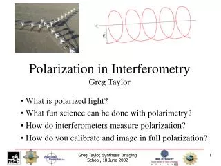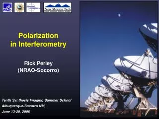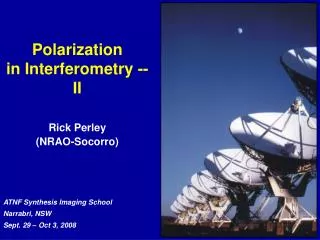
Polarization in Interferometry

1. Polarization in Interferometry Steven T. Myers (NRAO-Socorro)

2. Polarization in interferometry • Physics of Polarization • Interferometer Response to Polarization • Polarization Calibration & Observational Strategies • Polarization Data & Image Analysis • Astrophysics of Polarization • Examples • References: • Synth Im. II lecture 6, also parts of 1, 3, 5, 32 • “Tools of Radio Astronomy” Rohlfs & Wilson Polarization in Interferometry – S. T. Myers

3. WARNING! • Polarimetry is an exercise in bookkeeping! • many places to make sign errors! • many places with complex conjugation (or not) • possible different conventions (e.g. signs) • different conventions for notation! • lots of matrix multiplications • And be assured… • I’ve mixed notations (by stealing slides ) • I’ve made sign errors  (I call it “choice of convention” ) • I’ve probably made math errors  • I’ve probably made it too confusing by going into detail  • But … persevere (and read up on it later)  DON’T PANIC ! Polarization in Interferometry – S. T. Myers

4. Polarization Fundamentals Polarization in Interferometry – S. T. Myers

5. Physics of polarization • Maxwell’s Equations + Wave Equation • E•B=0 (perpendicular) ; Ez = Bz = 0 (transverse) • Electric Vector – 2 orthogonal independent waves: • Ex = E1 cos( k z – wt + d1 ) k = 2p / l • Ey = E2 cos( k z – wt + d2 ) w = 2pn • describes helical path on surface of a cylinder… • parameters E1, E2, d = d1 - d2 define ellipse Polarization in Interferometry – S. T. Myers

6. The Polarization Ellipse • Axes of ellipse Ea, Eb • S0 = E12 + E22 = Ea2 + Eb2 Poynting flux • dphase difference t = k z – wt • Ex = Ea cos ( t + d ) = Ex cos y + Ey sin y • Eh = Eb sin ( t + d ) = -Ex sin y + Ey cos y Rohlfs & Wilson Polarization in Interferometry – S. T. Myers

7. The polarization ellipse continued… • Ellipticity and Orientation • E1 / E2 = tan a tan 2y = - tan 2a cos d • Ea / Eb = tan c sin 2c = sin 2a sin d • handedness ( sin d > 0 or tan c > 0  right-handed) Rohlfs & Wilson Polarization in Interferometry – S. T. Myers

8. Polarization ellipse – special cases • Linear polarization • d = d1 - d2 = m pm = 0, ±1, ±2, … • ellipse becomes straight line • electric vector position angle y = a • Circular polarization • d = ½ ( 1 + m ) pm = 0, 1, ±2, … • equation of circle Ex2 + Ey2 = E2 • orthogonal linear components: • Ex = E cos t • Ey = ±Ecos ( t - p/2 ) • note quarter-wave delay between Ex and Ey ! Polarization in Interferometry – S. T. Myers

9. Orthogonal representation • A monochromatic wave can be expressed as the superposition of two orthogonal linearly polarized waves • A arbitrary elliptically polarizated wave can also equally well be described as the superposition of two orthogonal circularly polarized waves! • We are free to choose the orthogonal basis for the representation of the polarization • NOTE: Monochromatic waves MUST be (fully) polarized – IT’S THE LAW! Polarization in Interferometry – S. T. Myers

10. Linear and Circular representations • Orthogonal Linear representation: • Ex = Ea cos ( t + d ) = Ex cos y + Ey sin y • Eh = Eb sin ( t + d ) = -Ex sin y + Ey cos y • Orthogonal Circular representation: • Ex = Ea cos ( t + d ) = ( Er + El ) cos ( t + d ) • Eh = Eb sin ( t + d ) = ( Er - El ) cos ( t + d – p/2 ) • Er = ½ ( Ea + Eb ) • El = ½ ( Ea – Eb ) Polarization in Interferometry – S. T. Myers

11. The Poincare Sphere • Treat 2y and 2c as longitude and latitude on sphere of radius S0 Rohlfs & Wilson Polarization in Interferometry – S. T. Myers

12. Stokes parameters • Spherical coordinates: radius I, axes Q, U, V • S0 = I = Ea2 + Eb2 • S1 = Q = S0 cos 2c cos 2y • S2 = U = S0 cos 2c sin 2y • S3 = V = S0 sin 2c • Only 3 independent parameters: • S02 = S12 + S22 + S32 • I2 = Q2 + U2 + V2 • Stokes parameters I,Q,U,V • form complete description of wave polarization • NOTE: above true for monochromatic wave! Polarization in Interferometry – S. T. Myers

13. Stokes parameters and polarization ellipse • Spherical coordinates: radius I, axes Q, U, V • S0 = I = Ea2 + Eb2 • S1 = Q = S0 cos 2c cos 2y • S2 = U = S0 cos 2c sin 2y • S3 = V = S0 sin 2c • In terms of the polarization ellipse: • S0 = I = E12 + E22 • S1 = Q = E12 - E22 • S2 = U = 2 E1 E2 cos d • S3 = V = 2 E1 E2 sin d Polarization in Interferometry – S. T. Myers

14. Stokes parameters special cases • Linear Polarization • S0 = I = E2 = S • S1 = Q = I cos 2y • S2 = U = I sin 2y • S3 = V = 0 • Circular Polarization • S0 = I = S • S1 = Q = 0 • S2 = U = 0 • S3 = V = S (RCP) or –S (LCP) Note: cycle in 180° Polarization in Interferometry – S. T. Myers

15. Quasi-monochromatic waves • Monochromatic waves are fully polarized • Observable waves (averaged over Dn/n << 1) • Analytic signals for x and y components: • Ex(t) = a1(t) e i(f1(t) – 2pnt) • Ey(t) = a2(t) e i(f2(t) – 2pnt) • actual components are the real parts Re Ex(t), Re Ey(t) • Stokes parameters • S0 = I = <a12> + <a22> • S1 = Q = <a12> – <a22> • S2 = U = 2 < a1 a2 cos d > • S3 = V = 2 < a1 a2 sin d > Polarization in Interferometry – S. T. Myers

16. Stokes parameters and intensity measurements • If phase of Ey is retarded by e relative to Ex , the electric vector in the orientation q is: • E(t; q, e) = Ex cos q + Ey eie sin q • Intensity measured for angle q: • I(q, e) = < E(t; q, e) E*(t; q, e) > • Can calculate Stokes parameters from 6 intensities: • S0 = I = I(0°,0) + I(90°,0) • S1 = Q = I(0°,0) + I(90°,0) • S2 = U = I(45°,0) – I(135°,0) • S3 = V = I(45°,p/2) – I(135°,p/2) • this can be done for single-dish (intensity) polarimetry! Polarization in Interferometry – S. T. Myers

17. Partial polarization • The observable electric field need not be fully polarized as it is the superposition of monochromatic waves • On the Poincare sphere: • S02≥ S12 + S22 + S32 • I2≥ Q2 + U2 + V2 • Degree of polarization p : • p2 S02= S12 + S22 + S32 • p2 I2= Q2 + U2 + V2 Polarization in Interferometry – S. T. Myers

18. Summary – Fundamentals • Monochromatic waves are polarized • Expressible as 2 orthogonal independent transverse waves • elliptical cross-section  polarization ellipse • 3 independent parameters • choice of basis, e.g. linear or circular • Poincare sphere convenient representation • Stokes parameters I, Q, U, V • I intensity; Q,U linear polarization, V circular polarization • Quasi-monochromatic “waves” in reality • can be partially polarized • still represented by Stokes parameters Polarization in Interferometry – S. T. Myers

19. Antenna & Interferometer Polarization Polarization in Interferometry – S. T. Myers

20. Interferometer response to polarization • Stokes parameter recap: • intensity I • fractional polarization (pI)2= Q2 + U2 + V2 • linear polarization Q,U (mI)2= Q2 + U2 • circular polarization V (vI)2= V2 • Coordinate system dependence: • I independent • V depends on choice of “handedness” • V > 0 for RCP • Q,U depend on choice of “North” (plus handedness) • Q “points” North, U 45 toward East • EVPA F = ½ tan-1 (U/Q) (North through East) Polarization in Interferometry – S. T. Myers

21. Reflector antenna systems • Reflections • turn RCP  LCP • E-field allowed only in plane of surface • Curvature of surfaces • introduce cross-polarization • effect increases with curvature (as f/D decreases) • Symmetry • on-axis systems see linear cross-polarization • off-axis feeds introduce asymmetries & R/L squint • Feedhorn & Polarizers • introduce further effects (e.g. “leakage”) Polarization in Interferometry – S. T. Myers

22. Optics – Cassegrain radio telescope • Paraboloid illuminated by feedhorn: Polarization in Interferometry – S. T. Myers

23. Optics – telescope response • Reflections • turn RCP  LCP • E-field (currents) allowed only in plane of surface • “Field distribution” on aperture for E and B planes: Cross-polarization at 45° No cross-polarization on axes Polarization in Interferometry – S. T. Myers

24. Polarization field pattern • Cross-polarization • 4-lobed pattern • Off-axis feed system • perpendicular elliptical linear pol. beams • R and L beams diverge (beam squint) • See also: • “Antennas” lecture by P. Napier Polarization in Interferometry – S. T. Myers

25. Feeds – Linear or Circular? • The VLA uses a circular feedhorn design • plus (quarter-wave) polarizer to convert circular polarization from feed into linear polarization in rectangular waveguide • correlations will be between R and L from each antenna • RR RL LR RL form complete set of correlations • Linear feeds are also used • e.g. ATCA, ALMA (and possibly EVLA at 1.4 GHz) • no need for (lossy) polarizer! • correlations will be between X and Y from each antenna • XX XY YX YY form complete set of correlations • Optical aberrations are the same in these two cases • but different response to electronic (e.g. gain) effects Polarization in Interferometry – S. T. Myers

26. Example – simulated VLA patterns • EVLA Memo 58 “Using Grasp8 to Study the VLA Beam” W. Brisken Polarization in Interferometry – S. T. Myers

27. Example – simulated VLA patterns • EVLA Memo 58 “Using Grasp8 to Study the VLA Beam” W. Brisken Linear Polarization Circular Polarization cuts in R & L Polarization in Interferometry – S. T. Myers

28. Example – measured VLA patterns • AIPS Memo 86 “Widefield Polarization Correction of VLA Snapshot Images at 1.4 GHz” W. Cotton (1994) Circular Polarization Linear Polarization Polarization in Interferometry – S. T. Myers

29. Example – measured VLA patterns • frequency dependence of polarization beam : Polarization in Interferometry – S. T. Myers

30. Beyond optics – waveguides & receivers • Response of polarizers • convert R & L to X & Y in waveguide • purity and orthogonality errors • Other elements in signal path: • Sub-reflector & Feedhorn • symmetry & orientation • Ortho-mode transducers (OMT) • split orthogonal modes into waveguide • Polarizers • retard one mode by quarter-wave to convert LP  CP • frequency dependent! • Amplifiers • separate chains for R and L signals Polarization in Interferometry – S. T. Myers

31. Back to the Measurement Equation • Polarization effects in the signal chain appear as error terms in the Measurement Equation • e.g. “Calibration” lecture, G. Moellenbrock: Antenna i • F= ionospheric Faraday rotation • T = tropospheric effects • P = parallactic angle • E = antenna voltage pattern • D = polarization leakage • G = electronic gain • B = bandpass response Baseline ij (outer product) Polarization in Interferometry – S. T. Myers

32. Ionospheric Faraday Rotation, F • Birefringency due to magnetic field in ionospheric plasma • also present in radio sources! Polarization in Interferometry – S. T. Myers

33. Ionospheric Faraday Rotation, F • The ionosphere is birefringent; one hand of circular polarization is delayed w.r.t. the other, introducing a phase shift: • rotates the linear polarization position angle : • more important at longer wavelengths: • ionosphere most active at solar maximum and sunrise/sunset • watch for direction dependence (in-beam) • see “Low Frequency Interferometry” (C. Brogan) Polarization in Interferometry – S. T. Myers

34. Parallactic Angle, P • Orientation of sky in telescope’s field of view • Constant for equatorial telescopes • Varies for alt-az-mounted telescopes: • Rotates the position angle of linearly polarized radiation (c.f. F) • defined per antenna (often same over array) • P modulation can be used to aid in calibration Polarization in Interferometry – S. T. Myers

35. Parallactic Angle, P • Parallactic angle versus hour angle at VLA : • fastest swing for source passing through zenith Polarization in Interferometry – S. T. Myers

36. Antenna voltage pattern, E • Direction-dependent gain and polarization • includes primary beam • Fourier transform of cross-correlation of antenna voltage patterns • includes polarization asymmetry (squint) • can include off-axis cross-polarization (leakage) • convenient to reserve D for on-axis leakage • will then have off-diagonal terms • important in wide-field imaging and mosaicing • when sources fill the beam (e.g. low frequency) Polarization in Interferometry – S. T. Myers

37. Polarization Leakage, D • Polarizer is not ideal, so orthogonal polarizations not perfectly isolated • Well-designed systems have d < 1-5% • A geometric property of the antenna, feed & polarizer design • frequency dependent (e.g. quarter-wave at center n) • direction dependent (in beam) due to antenna • For R,L systems • parallel hands affected as d•Q + d•U , so only important at high dynamic range (because Q,U~d, typically) • cross-hands affected as d•Iso almost always important Leakage of q into p (e.g. L into R) Polarization in Interferometry – S. T. Myers

38. Coherency vector and correlations • Coherency vector: • e.g. for circularly polarized feeds: Polarization in Interferometry – S. T. Myers

39. Coherency vector and Stokes vector • Example: circular polarization (e.g. VLA) • Example: linear polarization (e.g. ATCA) Polarization in Interferometry – S. T. Myers

40. Visibilities and Stokes parameters • Convolution of sky with measurement effects: • e.g. with (polarized) beam E : • imaging involves inverse transforming these Instrumental effects, including “beam” E(l,m) coordinate transformation to Stokes parameters (I, Q, U, V) Polarization in Interferometry – S. T. Myers

41. Example: RL basis • Combining E, etc. (no D), expanding P,S: 2c for co-located array 0 for co-located array Polarization in Interferometry – S. T. Myers

42. Example: RL basis imaging • Parenthetical Note: • can make a pseudo-I image by gridding RR+LL on the Fourier half-plane and inverting to a real image • can make a pseudo-V image by gridding RR-LL on the Fourier half-plane and inverting to real image • can make a pseudo-(Q+iU) image by gridding RL to the full Fourier plane (with LR as the conjugate) and inverting to a complex image • does not require having full polarization RR,RL,LR,LL for every visibility • More on imaging ( & deconvolution ) tomorrow! Polarization in Interferometry – S. T. Myers

43. Leakage revisited… • Primary on-axis effect is “leakage” of one polarization into the measurement of the other (e.g. R  L) • but, direction dependence due to polarization beam! • Customary to factor out on-axis leakage into D and put direction dependence in “beam” • example: expand RL basis with on-axis leakage • similarly for XY basis Polarization in Interferometry – S. T. Myers

44. Example: RL basis leakage • In full detail: “true” signal 2nd order: D•P into I 2nd order: D2•I into I 1st order: D•I into P 3rd order: D2•P* into P Polarization in Interferometry – S. T. Myers

45. Example: Linearized response • Dropping terms in d2, dQ, dU, dV (and expanding G) • warning: using linear order can limit dynamic range! Polarization in Interferometry – S. T. Myers

46. Summary – polarization interferometry • Choice of basis: CP or LP feeds • Follow the Measurement Equation • ionospheric Faraday rotation F at low frequency • parallactic angle P for coordinate transformation to Stokes • “leakage” D varies with n and over beam (mix with E) • Leakage • use full (all orders) D solver when possible • linear approximation OK for low dynamic range Polarization in Interferometry – S. T. Myers

47. Polarization Calibration & Observation Polarization in Interferometry – S. T. Myers

48. So you want to make a polarization map… Polarization in Interferometry – S. T. Myers

49. Strategies for polarization observations • Follow general calibration procedure (last lecture) • will need to determine leakage D (if not known) • often will determine G and D together (iteratively) • procedure depends on basis and available calibrators • Observations of polarized sources • follow usual rules for sensitivity, uv coverage, etc. • remember polarization fraction is usually low! (few %) • if goal is to map E-vectors, remember to calculate noise in F= ½ tan-1 U/Q • watch for gain errors in V (for CP) or Q,U (for LP) • for wide-field high-dynamic range observations, will need to correct for polarized primary beam (during imaging) Polarization in Interferometry – S. T. Myers

50. Strategies for leakage calibration • Need a bright calibrator! Effects are low level… • determine gains G ( mostly from parallel hands) • use cross-hands (mostly) to determine leakage • general ME D solver (e.g. aips++) uses all info • Calibrator is unpolarized • leakage directly determined (ratio to I model), but only to an overall constant • need way to fix phase p-q (ie. R-L phase difference), e.g. using another calibrator with known EVPA • Calibrator of known polarization • leakage can be directly determined (for I,Q,U,V model) • unknown p-q phase can be determined (from U/Q etc.) Polarization in Interferometry – S. T. Myers