ScanSAR Interferometry
ScanSAR Interferometry. Jeremy Wurmlinger University of Kansas EECS826 Spring 2009. Topics. ScanSAR overview ScanSAR signal properties ScanSAR interferometry Spaceborne satellite ScanSAR Conclusion Questions/Comments?. ScanSAR overview. [1-4].

ScanSAR Interferometry
E N D
Presentation Transcript
ScanSAR Interferometry Jeremy Wurmlinger University of Kansas EECS826 Spring 2009
Topics • ScanSAR overview • ScanSAR signal properties • ScanSAR interferometry • Spaceborne satellite ScanSAR • Conclusion • Questions/Comments?
ScanSAR overview [1-4] • Also known as “Burst mode” or “Wide Swath mode” • Achieves a large swath coverage by periodically switching the antenna look angle • Changing Antenna look angle results in have Multiple Swath • During the look angle transfer, there is no transmit or receive(off period) • Allows imaging of a wide swath area at the expense of azimuth resolution • Typical swath widths range from 300km-500km • Raw data consists of bursts of radar echoes that are shorter than the synthetic aperature length • Various satellites are built with a ScanSAR mode: RADARSAT-1, RADARSAT-2, PALSAR among others.
ScanSAR overview [2] NB=Sequence of Burst Echo lines TB=Burst Duration TP=Burst Cycle Period T=Width of Antenna Footprint θ1=Look angle for first swath θ2=Look angle for second swath NL=T/TP (Burst Look: # of bursts per synthetic aperture) NS=TP/TB (# of possible subswaths)
ScanSAR Signal Properties Impulse Response of a point scatter Frequency Spectrum of a point scatterer [2] Strip-map mode [2] Strip-map mode [2] Burst mode [2] Burst mode
ScanSAR Signal Properties [1] Top figure-shows the raw data of a single point scatterer in strip mode Bottom figure-shows the raw data of the same scatterer in 4-burst mode
ScanSAR Signal Properties [1] Time frequency diagram of a single scatterer located at t=t0 WB=Burst Bandwidth WP=Distance between Spectral components of each individual burst WA=Chirp bandwidth HC(f;t0)=Signal Spectrum of the scatterer located at to
ScanSAR Signal Properties [1] Figure to the left depicts the impulse response in both strip and burst mode Figure to the right depicts the doppler centroid estimation of a scatterer in 2 Beam burst mode
ScanSAR Interferometry [1-3] • Multipass ScanSAR images may be used for interferogram generation to obtain elevation data • Several issues present themselves in inteferometric ScanSAR 1. Critical Baseline and Bandwidth 1. Doppler Centroid Estimation 2. PRF Ambiguity Resolution 3. Azimuth Scanning Pattern Synchronization 4. Range Processing 5. Azimuth Proecssing 6. Interferogram Generation
ScanSAR Interferometry [3] -Example of RADARSAT-1 datasheets used for Interferometry -Out of 12 RADARSAT datasets…two pairs existed with baseline shorter than critical baseline -Out of the 2 datasets, only 1 pair showed acceptable coherence -For DTM purposes, this particular ScanSAR dataset for RADARSAT was able to acheive better resolution than DTED-1
Burst Mode Image Products [1] Two Approaches to consider when approaching the phase-preserving data Single-Burst Image- Bursts are processed to individual complex images. The complex burst-mode product is then produced by these Burst complex images. Each image has a resolution to 1/WB and covers an azimuth extent of T-TB. One of the inconvenience asssociated with Single-Burst images are their azimuth-variant spectral bandpass characteristic. The signal varies linearly with azimuth from -WA/2 to WA/2 and wraps around several times in the +/- PRFn/2 band of the burst image This excludes the use of standard coregistration and resampling algorithms. Figure to the right shows the time frequency diagram of focused multiple burst RADARSAT ScanSAR data
Burst Mode Image Products [1] Multiple-Burst Image- involves the coherent superposition of the burst images forming a single full-aperture image. Suffers the multiple peak shape of figure in the right hand corner. It has been shown, however that a low-pass filter applied to the multiple-burst image gives a image comparable to the one obtained by incoherent superposition of burst images. The average spectral envelope of such a complex burst image is identical to that of a strip-map mode. Therefore, standard InSAR processing can be applied to multiple-burst images. The cost of this however is increased data volume. [3]
Critical Baseline and Bandwidth [1-2] Critical Baselines for RADARSAT modes and ERS -ScanSAR typically operates in a reduced range chirp bandwidth -Not only a resolution problem, but also effects the size of the critical baseline -Core reason why Narrow beam mode is preferred when using ScanSAR for Interferometric purposes -A lower range chirp bandwidth also requires tighter margins for repeated orbit trajectories (Critical Baseline increases with increase in incidence angle)
-Since the shape of the doppler spectrum will be distorted in Burst mode….Doppler Centroid estimation is more difficult than Stripmap mode. Doppler Centroid [1] [5] -Can be achieved by packing the bursts densely in the azimuth direction, which would give an uninterrupted sequence of range lines…then pass through a Doppler Centroid Estimator(same as strip mode) Yaw Steering- Antenna mid-beam axis is pointed in the direction of the Zero Doppler frequency. This results in the majority of the Doppler Centroid values being the 0th PRF band. -Allows coregistration parameters to be derived for each individual swath -Avoids Phase biases due to interferometric misregistration, PRF ambiguity resolution,and Beam alignment and baseline estimate become much easier
PRF Ambiguity [1] If a satellite in not yaw-steered, then PRF ambiguity resolution is necessary. Without the use of Yaw Steering….Doppler Centroid Values exceeding +-PRF/2 are expected Various methods can be applied to compensate for the PRF ambiguity. As discussed in Holzner and Bamler’s, a range look correlation technique is used. Since ScanSAR scenes cover areas about 10 times as large strip-map images, it is very likely that there are a few point targets in the scene. With the range look correlation, these point-like targets will be automatically detected. [1] The figure to the right shows the range Cross correlation of two looks of a point like target.
Azimuth Scanning Pattern Synchronization [1-2] • Azimuth Scanning Pattern-azimuth pattern of the sequence of bursts(radar on) and pauses(radar off) • Interferogram formation requires that the burst patterns of both datasets be aligned with each other • The goal of Azimuth Scanning Pattern Synchronization is to perserve companions of raw data lines of the same ground area located in your image. • poses a problem when trying to perform interferometric processing • Another reason why narrow beam ScanSAR is preferred over wide beam ScanSAR. [3] Figure to the right shows the variation of interferogram peak values vs mutual azimuth shift. The large peak indicates a high ASPS. The figure was formed from the method discussed on next slide. [1]
Azimuth Scanning Pattern Synchronization [1-2] Pre-Processing Method • Small azimuth portion of both image datasets is taken • Mutual azimuth shift is estimated from the two images • Co-registration of the two datasets(accuracy to 1 range line) • Only the range lines that related in for both datasets are kept for further processing; the rest are discarded. The more in sync the burst cycles of each dataset are with each other, the finer the final azimuth resolution of the interferometric image will be. “Mutually exclusive”-on cycles of one dataset line up with off cycles of the second dataset [1-2] [3]
Range Processing [1-2] Two methods of Range Processing are but not limited to: -Single Burst Range Processing -Pack and Go Range Processing(proposed by Holzner and Balmer) Single Burst Range Processing-Each burst of range lines is processed separately by a standard processor whose azimuth compression has been disabled. This method is computationally efficient, however, often the bursts must be supplemented by a number of range lines containing zeroes to the next power of two. [1]
Range Processing [1] Pack & Go Range Processing-Since during range processing (almost) no energy leakage in azimuth occurs, several bursts can be concatenated (with a few zero-lines as “safety margins” separating the different bursts) and processed simultaneously by the standard SAR processor.. This method is more efficient than single-burst processing, since arbitrarily long FFTs can be used and zero padding (to meet the power-of-two requirement) is negligible. Existing strip-map SAR processors can be used like a black box, no matter how large their internally used azimuth processing blocks are. Also Doppler centroid estimation that uses large estimation windows can be conveniently applied to this packed burst dataset. [1] [9]
Azimuth Processing [1] A focused burst image exhibits a range-dependent azimuth sample spacing known as fan-shape distortion. When performing Azimuth processing, an additional interpolation step is required. Azimuth Variant Filtering -After a burst has been range processed, standard azimuth compression is applied. The result is a coherent superposition of several shifted replicas of the desired burst image.A time-domain azimuth band-pass filter whose center frequency varies with azimuth position is required finally to separate the correct result from the aliased one. Extend Chirp Scaling- One method used to avoid the fan-shape distortion and the additional interpolation step could be done by using a high precision ECS algorithm, which would use the standard SPECAN method for the azimuth processing and the chirp scaling for accurate range processing. Adding a azimuth scaling step would also equalize the frequency rates of the azimuth chirps. Time-Domain Azimuth Correlation-Since the bursts are usually short, a straightforward time-domain azimuth correlation is an alternative to frequency domain methods. Although not as efficient, it is most easily implemented and allows for a free choice of the output sample spacing. [3]
Single Burst Images -Burst Images acquired from each pass -Individual Burst interferograms formed -Arrangement of Burst interferograms to form subswath interferograms -Arrange subswath interferograms to form NL interferograms Multiple Burst Images -Multiple Burst images are stored -Coherently add each individual burst image from each pass over the target area. -Interferogram formation -Low-Pass filter -NL interferogram is formed Phase Preserving Burst Mode Processing [2] Final Interferogram formation essentially equivalent whether from Single Burst method or Multiple Burst Method
Single-Burst Interferogram Method [2] Companion Burst Images acquired from each pass Individual ‘Burst’ Interferograms are formed Subwath Inteferogram formed by coherent addition of each burst interferogram Arrange subwath interferograms to obtain the NL interferogram [2]
Multi-Burst Interferogram Method [2] Multiple Burst images are stored for each Pass(N=3) Coherent addition of each individual burst image from each pass to form a multiple burst image Interferogram is formed Low-Pass filtering NL interferogram is formed [2]
Multi-Looking [1-3] For the generation of subswath interferograms, the singleburst interferograms are coherently mosaicked. Straightforward multi-looking requires that the bursts are processed to the same grid within and across beams. Usually, the PRFs in the individual beams differ; hence, the raw data echo lines of the bursts within one swath are not acquired on a continuous integer pixel grid. The ScanSAR processor should arrange the data on a common reference grid to facilitate further processing. Differential interferograms generated between bursts within one subswath can be used to identify phase and sampling errors. [2]
Re-Sampling [1-2] Mutual registration of the interferometric partners requires interpolation of the signal at inter-pixel positions. For multiple and single-burst images sampled at the acquisition PRF, conventional interpolation methods can be applied since at the large PRF, the average burst signal spectrum resembles the one of strip-map data Depending on the sampling frequency, single-burst image re-sampling has to account for the azimuth variant band-pass behavior of the signal. Technique proposed Holzner and Bamler 1. Burst Signal is de-ramped by a quadratic phase function in the time domain such that a low pass signal is obtained 2. The low pas signal is then re-sampled using standard interpolation algorithm 3. The Quadratic phase is removed for further processing Alternative approach would be to apply azimuth-varying band pass for resampling.
Beam Alignment [1-2] The swath interferograms can be either processed to individual DEMs or first combined to a full-swath interferogram and then processed to a single DEM. The swath overlap region provides valuable information on swath registration and mutual phase offsets of the interferograms. Swath co-registration can be verified by cross-correlation of homologous patches on an image contrast basis. Misalignment in range will not only disturb topographic information after swath interferogram combination but also generates a phase offset owing to the dominant (“flat earth”) fringe frequency of the swath interferograms. High Doppler centroid values, together with tiny misregistration of the interferometric partners will generate slowly varying phase errors that also affect the overlap area of the swath interferograms.
Satellite Orbit Drift Satellite Orbit Data, such as RADARSAT, can have low accuracy. ScanSAR interferometry is optimal under certains conditions. For RADARSAT-1 The westward drift lies within ±4 km, and the orbit boosts occur approximately every 35 days. The minimum drift rate of the satellite occurs halftime between boosts at the drift maximum. Acquisitions around this minimum drift rate are favorable for ScanSAR interferometry since baselines are expected to be within the critical baseline. Alternatively, Orbit Correction can be split into two tasks. • Correct the primary channel orbit for shifts in slant range and azimuth direction • Correcting the secondary channel optimize the baseline length and orbit angle. [1]
Satellite Orbit Drift [2] [2]
RADARSAT-1 [10-11] RADARSAT-1 was launched at 14h22 on November 4, 1995 from Vandenberg AFB in California, into a sun-synchronous orbit(dawn-dusk) above the Earth with an altitude of 798 kilometers and inclination of 98.6 degrees. Developed under the management of the CSA in cooperation with Canadian provincial governments and the private sector, it provides images of the Earth for both scientific and commercial applications. NASA provided the Delta II rocket to launch RADARSAT-1 in exchange for access to its data. Estimates are that the project, excluding launch, cost $620 million (Canadian). The Canadian federal government contributed about $500 million, the four participating provinces (Quebec, Ontario, Saskatchewan, and BC) about $57 million, and the private sector about $63 million It C-Band satellite that operates at 5.3GHz and has the ability of a ScanSAR mode that provides potential swath widths up to 500km. While it used to achieve high quality images of the earth, it has the flexibility to support specific requirements.
RADARSAT-1 [10-11] The RADARSAT-1 SAR utilizes beam forming techniques in order to provide several different beam modes. The modes may be capable of imaging closer to or farther from the satellite, with finer resolution and accordingly smaller areas or wide areas with worse resolution. RADARSAT-1 ScanSAR mode actually combines a few of these other modes in order to obtain a very wide swath - approximately 500 km, depending on which ScanSAR sub-mode is chosen. Three resolutions are provided: 75, 150, and 600 meters ScanSAR(Narrow mode) -~250km nadir offset -~400km nadir offset -Swath width: 300km -Range Resolution: 50m -Azimuth Resolution: 50m -Look(s): 2-4 -Incidence Angle: 20-40°,32-46° ° ScanSAR(Wide mode) -~250km nadir offset -Swath width: 500km,440km -Range Resolution: 100m -Azimuth Resolution: 100m -Look(s): 4-8 -Incidence Angle: 20-50°
RADARSAT-2 [11] RADARSAT-2 was successfully launched on December 14 of 2007 for the CSA by Starsem, using a Soyuz FG launch vehicle. It was developed to be a follow-on to RADARSAT-1. It has the same orbit (798Km orbit) and is separated by half an orbit period from RADARSAT-1. Also operating in C-band, RADARSAT-2 was designed to support all existing RADARSAT-1modes and offers higher quality features ranging from improvement in resolution, to full flexibility in the selection of polarization options. [13] Key Features and Benefits -C-Band(5.405GHz) -3-100 meter resolution -HH,HV,VV,VH channel polarization -Left and Right Looking operation -Solid-State Recorders -On-Board GPS receivers -Yaw-Steering capable -Reduced programing lead time -Rapid tasking and priority programming levels -Improved processing abilities and speed -ScanSAR Wide-500km swath width 100m*100m resolution 20-49° incidence angle Single or Dual polariztion -ScanSAR Narrow-300km swath width 50m*50m resolution 20-46° incidence angle Single or Dual polarization
RADARSAT-2 RADARSAT-2 ScanSAR Wide Mode(VV,VH) Brazil, March 3,2008 [14]
RADARSAT-2 RADARSAT-2 ScanSAR Narrow Mode(VV,VH) Thunder Bay, Ontario, Canada March 3rd 2008 [15]
ALOS PALSAR [7] The Advanced Land Observing Satellite (ALOS), launched on 24 January 2005, is a joint project between JAXA and the Japan Resources Observation System Organization (JAROS). ALOS has three remote-sensing instruments: the Panchromatic Remote-sensing Instrument for Stereo Mapping (PRISM) for digital elevation mapping, the Advanced Visible and Near Infrared Radiometer type 2 (AVNIR-2) for precise land coverage observation, and the Phased Array type L-band Synthetic Aperture Radar (PALSAR) for day-and-night and all-weather land observation.
ALOS PALSAR [16] With a wavelength of 23.6cm, PALSAR can obtain swath widths up to 350km while retaining a spatial resolution of 71-157m*100m(az) at 5 scan, short burst. [17]
Shuttle Radar Topography Mission(SRTM) [18] • In February of 2000, the space shuttle Endeavor carried a specially modified Radar system on a 11 day mission. • Obtained elevation data on a near-global scale to generate the most complete high resolution digital topographic database of the earth. • Only the use of ScanSAR interoferometry made it possible to map 80% of the earth’s landmass.
Shuttle Radar Topography Mission(SRTM) [18] • C-Band Antenna used Four Beam ScanSAR narrow mode to form 225km swath widths • Illuminated two subswaths at a time using orthogonal polarizations • By use of it’s polarimetric abilities, the ScanSAR duty cycle was 2:1 rather than 4:1 • The X-band antenna did not have steering cababilities and has to operate at a fixed nadir look angle of 52° and swath width of about 45km • The X-band antenna was able to provide higher relative height accuracies by a factor of 2; but could not come close to the coverage that the C-Band ScanSAR was able to provide
Shuttle Radar Topography Mission(SRTM) • To obtain the DTM data the system was equipped with two antennas. • One antenna was located inside the payload bay of the shuttle, while the other was located on one end of a 200ft mast that extended from the payload out into space. • Terrain Data that was mapped was located between 60 degrees North latitude and 54 degrees south latitude.
Shuttle Radar Topography Mission(SRTM) [18] SRTM main antenna -Consists of two antennas: X-band and C-band -C-Band Antenna used for the SRTM mission -Both Transmit and receive antenna -5.6cm wavelength -225km swath width
Shuttle Radar Topography Mission(SRTM) [18] SRTM outboard antenna -Consists of: X-Band and C-Band antennas, two GPS antennas, LED targets,and a corner cube reflector -Only receive antenna; main antenna used for transmit -mast was extended ~60m from the main antenna
Conclusion The future of InSAR is highly dependent upon the ScanSAR interferometry and the continued launch of satellites with ScanSAR capabilites. While sacrificing spatial resolution for swath width is the cost of ScanSAR, future technology and processing continues to grow and show finer resolutions with each new spaceborne satellite. The ability to produce DEMs on a World wide coverage in a minimial amount of time is a highly valuable resource. Which is one of the reasons why ScanSAR mode has become a standard SAR mode on current and future spaceborne satellite missions. As discussed, the ScanSAR interferometry introduces many complications that the standard strip map mode does not have. The variations in the methods and processes used to work around this complications are not defined and are up to the Individual on how they would like to process that data. New algorithms and processing techniques are being continuously to achieve the finer resolutions at the higher swath widths.
References [1]Bamler, Richard and Holzner, Jurgen, “Burst-Mode and ScanSAR Interferometry”, IEEE Transactions on Geoscience and Remote Sensing, Vol 40, No. 9, September 2002 [2]Bamler, Richard and Holzner, Jurgen, “ScanSAR Interferometry for RADARSAT -2&3”, Can. J. Remote Sensing, Vol 30, No. 3, pp. 437-447, 2004 [3]Bamler, Richard and Holzner, Jurgen, “RADARSAT ScanSAR Interferometry”, Geoscience and Remote Sensing Symposium, 1999. IGARSS ’99 Proceedings, Vol 3, July 1999 [4]Guarnieri, Andrea Monti and Prati, Claudo, “ScanSAR Focusing and Interferometry”, IEEE Transactions on Geoscience and Remote Sensing, Vol 34, No. 4, July 1996 [5]Jin, Michael, “Optimal Range and Doppler Centroid Estimation for a ScanSAR System”, IEEE Transactions on Geoscience and Remote Sensing, Vol 34, No. 2, pp. 479-488, March 1996 [6]Tomiyasu,Kiyo,”Conceptual Performance of a Satellite Borne Wide Swath Synthetic Aperature Radar”, IEEE Transactions on Geoscience and Remote Sensing, Vol GGE-19, No. 2, pp. 108-118, April 1981 [7]Shimada, M.A.R and Watanabe Manabe, “ALOS PALSAR: Technical Outline and mission concepts”, 4th International Symposium on Retrieval of Bio- and Geophysical Parameters from SAR Data for Land Applications”, Innsbruck, Austria, Nov 16-19,2004 [8]Bamler, Richard,”The SRTM Mission: A World-Wide 30m Resolution DEM from SAR Interferometry in 11 Days”, Photogrammetric Week ’99’, 1999 [9]http://earth.esa.int/dragon/symp2008/proceedings/38jia.pdf [10]http://www.asc-csa.gc.ca/eng/satellites [11]http://cct.rncan.gc.ca/radar/spaceborne/radarsat1/specs/radspec_e.php [12]http://envisat.esa.int/handbooks/asar/CNTR2-6-1-2-4-2.htm [13]http://www.imagingnotes.com/ee_assets/2008_fall/radarsat-2-f06.jpg [14]http://www.radarsat2.info/images/gallery/RSAT-2_ScanSAR_Brazil.jpg [15]http://www.radarsat2.info/images/gallery//RSAT-2_ScanRAR_Thunder_Bay.jpg [16]http://www.palsar.ersdac.or.jp/ [17]http://earth.esa.int/object/index.cfm?fobjectid=5198 [18]http://www2.jpl.nasa.gov/srtm/radaroverview.html