Understanding Principles of Interferometry in Radio Astronomy
500 likes | 613 Vues
Delve into the basics of interferometry, coherence characteristics, and signal multiplication in radio astronomy, exploring the response from extended sources.

Understanding Principles of Interferometry in Radio Astronomy
E N D
Presentation Transcript
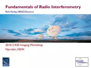
Principles of Interferometry Rick Perley National Radio Astronomy Observatory Socorro, NM
Topics • Setting the Stage -- Coherence • The Quasi-Monochromatic, Stationary Interferometer • Visibility and its relationship to Brightness • Coordinate Systems • The Consequences of Finite Bandwidth • Adding Time Delay and Source Motion • The Consequences of Finite Time Averaging • Frequency Conversions – The Magic of Heterodyning Eleventh Synthesis Imaging Workshop, June 10-17, 2008
In a Galaxy, Far, Far Away … • A source of emission radiates an EM wave, which passes by a planet inhabited by sentient, curious beings who, being technically competent, build sensors (a.k.a. ‘antennas’) which allow them to collect, and analyze, this radiation. • Understanding that they cannot build an antenna large enough to satisfy their curiosity about the structure of distant emission, they wonder if they can achieve their goals by analyzing the signals collected by pairs of widely-separated antennas. • What are the coherence characteristics of the EM wave as a function of spatial separation? Is there information about the angular structure of the emission encoded in the coherence properties, and if so, how can it be extracted? Eleventh Synthesis Imaging Workshop, June 10-17, 2008
Establishing Some Basics • Consider radiation from direction s from a small elemental solid angle, dW, at frequency n within a frequency slice, dn. • For sufficiently small dn, the electric field properties (amplitude, phase) are stationary over timescales of interest (seconds), and we can write the field as • The purpose of an antenna and its electronics is to convert this E-field to a voltage, V(t) – proportional to the amplitude of the electric field, and which preserves the phase of the E-field – which can be conveyed from the collection point to some other place for processing. • We ignore the gain of the electronics and the collecting area of the antennas – these are calibratable items (‘details’). • The coherence characteristics can be analyzed through consideration of the dependencies of the product of the voltages from the two antennas. Eleventh Synthesis Imaging Workshop, June 10-17, 2008
The Stationary, Quasi-Monochromatic Interferometer • Consider radiation from a small solid angle dW, from direction s, at frequency n, within dn: s s Geometric Time Delay The path lengths from antenna to correlator are assumed equal. b.s b An antenna X multiply average
Examples of the Signal Multiplications The two input voltages are shown in red and blue, their product is in black. The desired coherence is the average of the black trace. In Phase:wtg = 2pn Quadrature Phase: wtg=(2n+1)p/2 Anti-Phase: wtg= (2n+1)p Eleventh Synthesis Imaging Workshop, June 10-17, 2008
Signal Multiplication, cont. • The averaged product RC is dependent on the source power, A2 and geometric delay, tg: • RC is thus dependent only on the source strength, location, and baseline geometry. • RC is not a a function of: • The time of the observation (provided the source itself is not variable!) • The location of the baseline, provided the emission is in the far-field. • The strength of the product is also dependent on the antenna areas and electronic gains – but these factors can be calibrated for. • We identify the product A2 with the specific intensity (or brightness) In of the source within the solid angle dW and frequency slice dn. Eleventh Synthesis Imaging Workshop, June 10-17, 2008
The Response from an Extended Source • The response from an extended source is obtained by summing the responses for each antenna over the sky, multiplying, and averaging: • The expectation, and integrals can be interchanged, and providing the emission is spatially incoherent, we get • This expression links what we want – the source brightness on the sky, In(s), – to something we can measure - RC, the interferometer response. Eleventh Synthesis Imaging Workshop, June 10-17, 2008
A Schematic Illustration • The correlator can be thought of ‘casting’ a sinusoidal coherence pattern, of angular scalel/b radians, onto the sky. • The correlator multiplies the source brightness by this coherence pattern, and integrates (sums) the result over the sky. • Orientation set by baseline geometry. • Fringe separation set by (projected) baseline length and wavelength. • Long baseline gives close-packed fringes • Short baseline gives widely-separated fringes • Physical location of baseline unimportant, provided source is in the far field. l/b rad. Source brightness - + - + - + - Fringe Sign Eleventh Synthesis Imaging Workshop, June 10-17, 2008
Odd and Even Functions • But the measured quantity, Rc, is insufficient – it is only sensitive to the ‘even’ part of the brightness, IE(s). • Any real function, I(x,y), can be expressed as the sum of two real functions which have specific symmetries: An even part: An odd part: IE IO I = + Eleventh Synthesis Imaging Workshop, June 10-17, 2008
Why Two Correlations are Needed • The integration of the cosine response, Rc, over the source brightness is sensitive to only the even part of the brightness: since the integral of an odd function (IO) with an even function (cos x) is zero. • To recover the ‘odd’ part of the intensity, IO, we need an ‘odd’ fringe pattern. Let us replace the ‘cos’ with ‘sin’ in the integral: since the integral of an even times an odd function is zero. • To obtain this necessary component, we must make a ‘sine’ pattern. Eleventh Synthesis Imaging Workshop, June 10-17, 2008
Making a SIN Correlator • We generate the ‘sine’ pattern by inserting a 90 degree phase shift in one of the signal paths. s s b.s b An antenna X 90o multiply average
Define the Complex Visibility • We now DEFINE a complex function, V, from the two independent correlator outputs: where • This gives us a beautiful and useful relationship between the source brightness, and the response of an interferometer: • Although it may not be obvious (yet), this expression can be inverted to recover I(s) from V(b). Eleventh Synthesis Imaging Workshop, June 10-17, 2008
The Complex Correlator • A correlator which produces both ‘Real’ and ‘Imaginary’ parts – or the Cos and Sin fringes, is called a ‘Complex Correlator’ • For a complex correlator, think of two independent sets of projected sinusoids, 90 degrees apart on the sky. • In our scenario, both are necessary, because we have assumed there is no motion – the ‘fringes’ are fixed on the source emission. • One can use a single correlator if the inserted phase alternates between 0 and 90 degrees, or if the phase cycles through 360 degrees. • Or, let the source drift through the fringes. • In this case, there will be a sinusoidal output from the correlator, whose amplitude and phase define the Visibility. Eleventh Synthesis Imaging Workshop, June 10-17, 2008
Picturing the Visibility • The intensity, In, is in black, the ‘fringes’ in red. The visibility is the integral of the product – the net dark green area. RC RS Long Baseline Short Baseline
Basic Characteristics of the Visibility • For a zero-spacing interferometer, we get the ‘single-dish’ (total-power) response. • As the baseline gets longer, the visibility amplitude will in general decline. • When the visibility is close to zero, the source is said to be ‘resolved out’. • Interchanging antennas in a baseline causes the phase to be negated – the visibility of the ‘reversed baseline’ is the complex conjugate of the original. • Mathematically, the Visibility is Hermitian, because the Brightness is a real function. Eleventh Synthesis Imaging Workshop, June 10-17, 2008
Comments on the Visibility • The Visibility is a function of the source structure and the interferometer baseline length and orientation. • Each observation of the source with a given baseline length and orientation provides one measure of the visibility. • Sufficient knowledge of the visibility function (as derived from an interferometer) will provide us a reasonable estimate of the source brightness. Eleventh Synthesis Imaging Workshop, June 10-17, 2008
Geometry – the perfect, and not-so-perfect To give better understanding, we now specify the geometry. Case A: A 2-dimensional measurement plane. Let us imagine the measurements of Vn(b) to be taken entirely on a plane. Then a considerable simplification occurs if we arrange the coordinate system so one axis is normal to this plane. Let (u,v,w) be the coordinate axes, with w normal to the plane. All distances are measured in wavelengths. The components of the unit direction vector, s, are: and for the solid angle Eleventh Synthesis Imaging Workshop, June 10-17, 2008
Direction Cosines w The unit direction vectors is defined by its projections on the (u,v,w) axes. These components are called the Direction Cosines. s n q b a v m l b u The baseline vectorbis specified by its coordinates (u,v,w) (measured in wavelengths). In this special case, Eleventh Synthesis Imaging Workshop, June 10-17, 2008
The 2-d Fourier Transform Relation Then,nb.s/c = ul + vm + wn = ul + vm, from which we find, which is a2-dimensional Fourier transformbetween the projected brightness and the spatial coherence function (visibility): And we can now rely on a century of effort by mathematicians on how to invert this equation, and how much information we need to obtain an image of sufficient quality. Formally, With enough measures of V, we can derive an estimate of I. Eleventh Synthesis Imaging Workshop, June 10-17, 2008
Interferometers with 2-d Geometry • Which interferometers can use this special geometry? a) Those whose baselines, over time, lie on a plane (any plane). All E-W interferometers are in this group. For these, the w-coordinate points to the NCP. • WSRT (Westerbork Synthesis Radio Telescope) • ATCA(Australia Telescope Compact Array) • Cambridge 5km telescope (almost). b) Any coplanar 2-dimensional array, at a single instance of time. • VLA or GMRTin snapshot (single short observation) mode. • What's the ‘downside’ of 2-d arrays? • Full resolution is obtained only for observations that are in the w-direction. • E-W interferometers have no N-S resolution for observations at the celestial equator. • A VLA snapshot of a source will have no ‘vertical’ resolution for objects on the horizon. Eleventh Synthesis Imaging Workshop, June 10-17, 2008
3-d Interferometers Case B: A 3-dimensional measurement volume: • What if the interferometer does not measure the coherence function on a plane, but rather does it through a volume? In this case, we adopt a different coordinate system. First we write out the full expression: (Note that this is not a 3-D Fourier Transform). • Then, orient the coordinate system so that the w-axis points to the center of the region of interest, u points east and v north, and make use of the small angle approximation: where q is the polar angle from the center of the image. • The w-component is the ‘delay distance’ of the baseline. Eleventh Synthesis Imaging Workshop, June 10-17, 2008
VLA Coordinate System w points to the source, u towards the east, and v towards the north. The direction cosines l and m then increase to the east and north, respectively. w s0 s0 b v Eleventh Synthesis Imaging Workshop, June 10-17, 2008
3-d to 2-d With this choice, the relation between visibility and intensity becomes: The quadratic term in the phase can be neglected if it is much less than unity: Or, in other words, if the maximum angle from the center is: (angles in radians!) then the relation between the Intensity and the Visibility again becomes a 2-dimensional Fourier transform: Eleventh Synthesis Imaging Workshop, June 10-17, 2008
3-d to 2-d where the modified visibility is defined as: and is, in fact, the visibility we would have measured, had we been able to put the baseline on the w = 0 plane. • This coordinate system, coupled with the small-angle approximation, allows us to use two-dimensional transforms for any interferometer array. • Remember that this is an approximation! The visibilities really are measured in a volume, and projecting them onto the ‘normal plane’ results in imaging distortions that increase with polar angle. • How do we make images when the small-angle approximation breaks down? That's a longer story, for another day. Short answer: we know how to do this, and it takes a lot more computing). Eleventh Synthesis Imaging Workshop, June 10-17, 2008
Examples of Brightness and Visibilities Eleventh Synthesis Imaging Workshop, June 10-17, 2008
More Examples of Visibility Functions • Top row: 1-dimensional even brightness distributions. • Bottom row: The corresponding real, even, visibility functions. In(l) V(u) Eleventh Synthesis Imaging Workshop, June 10-17, 2008
The Effect of Bandwidth. • Real interferometers must accept a range of frequencies. So we now consider the response of our interferometer over frequency. • To do this, we first define the frequency response functions, G(n), as the amplitude and phase variation of the signal over frequency. • The function G(n) is primarily due to the gain and phase characteristics of the electronics, but will also contain propagation path effects. Dn G n n0 Eleventh Synthesis Imaging Workshop, June 10-17, 2008
The Effect of Bandwidth. • Providing the emission is frequency incoherent, we simply integrate our fundamental response over a frequency width Dn, centered at n0: If the source intensity does not vary over the bandwidth, and the instrumental gain parameters G are square and real, then The fringe attenuation function, sinc(x), is defined as: Eleventh Synthesis Imaging Workshop, June 10-17, 2008
The Bandwidth/FOV limit • This shows that the source emission is attenuated by the spatially variant function sinc(x), also known as the ‘fringe-washing’ function. • The attenuation is small when: which occurs when (exercise for the student) • The ratioDn/nis the fractional bandwidth, typically 1/25. • The ratioq/qresis the source offset in units of the fringe separation,qres = l/b. • This ratio can be as large as ~ B/D – a value in the thousands. Eleventh Synthesis Imaging Workshop, June 10-17, 2008
Bandwidth Effect Example • For a square bandpass, the bandwidth attenuation reaches a null at an angle equal to the fringe separation multiplied by n0/Dn. • If Dn = 60 MHz, and B = 30 km, then the null occurs at about 1 degree off the meridian. Envelope function: Eleventh Synthesis Imaging Workshop, June 10-17, 2008
Observations off the Meridian • The present analysis shows that only observations of small-diameter objects on meridian transit can be made without bandwidth attenuation. For arrays with different baseline orientations, this means at the zenith only! • So: How can we observe an object at a different position, without suffering these bandwidth attenuation? • One solution is to use a very narrow bandwidth – this loses sensitivity, which can only be made up by utilizing many channels – feasible, but computationally expensive. • Better answer: Shift the fringe-attenuation function to the center of the source of interest. • How? By adding time delay. Eleventh Synthesis Imaging Workshop, June 10-17, 2008
Adding Time Delay s0 s0 s s S0 = reference direction S = general direction t0 tg b An antenna X t0 Eleventh Synthesis Imaging Workshop, June 10-17, 2008
Coordinates • The insertion of this delay centers both the fringes and the bandwidth delay pattern about a cone defined byt-tg= 0. The width of field of view is as before: Dq/qres< n/Dn • Remembering the coordinate system discussed earlier, where the w axis points to the reference center (s0), assuming the introduced delay is appropriate for this center, and that the bandwidth losses are negligible, we have: Eleventh Synthesis Imaging Workshop, June 10-17, 2008
Reduction to a 2-d Fourier Transform • Inserting these, we obtain: • The third term in the exponential is generally very small, and can be ignored in many cases, as discussed before, giving • Which is again a 2-dimension Fourier transform between the visibility and the projected brightness. Eleventh Synthesis Imaging Workshop, June 10-17, 2008
Observations from a Rotating Platform • Real interferometers are built on the surface of the earth – a rotating platform. • Since we know how to adjust the interferometer to move its reception pattern to the direction of interest, it is a simple step to move the pattern to follow a moving source. • All that is necessary is to continuously slip the inserted time delay. • For the ‘radio-frequency’ interferometer we are discussing here, this will automatically track both the fringe pattern and the fringe-washing function with the source. • Hence, a point source, at the reference position, will give uniform amplitude and zero phase throughout time (provided real-life things like the atmosphere, ionosphere, or geometry errors don’t mess things up … ) Eleventh Synthesis Imaging Workshop, June 10-17, 2008
Coverage of the U-V Plane • The advantage of building an interferometer on a rotating platform is that you don’t need to move the antennas to measure more Fourier components. • If the platform is the earth, how does the (u,v) plane fill up? • Adopt an earth-based coordinate grid to describe the antenna positions: • X points to H=0, d=0 (intersection of meridian and celestial equator) • Y points to H = -6, d = 0 (to east, on celestial equator) • Z points to d = 90 (to NCP). • Then denote by (Lx, Ly, Lz) the coordinates of a baseline. Eleventh Synthesis Imaging Workshop, June 10-17, 2008
(U,V) Coordinates • Then, it can be shown that • The u and v coordinates describe E-W and N-S components of the projected interferometer baseline. • The w coordinate is the delay distance, in wavelengths between the two antennas. The geometric delay, tgis given by • Its derivative, called the fringe frequency nFis of vital importance: Eleventh Synthesis Imaging Workshop, June 10-17, 2008
Sample (U,V) plots for 3C147 (d = 50) • Snapshot (u,v) coverage for HA = -2, 0, +2 HA = 0h HA = -2h HA = 2h Coverage over all four hours. Eleventh Synthesis Imaging Workshop, June 10-17, 2008
Time-Averaging Loss • The downside of a rotating platform is that not all objects in the sky move at the same rate. • We can only insert delay, and track the fringes, for one direction – for all others, the sources are differentially moving through the fringes. • This `problem’ has a practical consequence – if we integrate the output too long, the visibility amplitudes will be attenuated. • For simplicity, consider the reference position at the north pole, and the target position a small angle q away. A source at this distance travels at a rate of qwe radians/sec. ( we = angular rotation rate of the earth = 7 x 10⁻⁵ rad/sec). • If the fringe separation for this object is l/B radians, then it takes t =l/(Bqwe) seconds for the object to move through the pattern. • Worst case: q ~ l/D, so t ~ D/(Bwe) seconds. (10 sec for A-config.) Eleventh Synthesis Imaging Workshop, June 10-17, 2008
Time-Smearing Loss • Simple derivation of fringe period, from observation at the NCP. • Light blue area is antenna primary beam on the sky – radius = l/D • Interferometer coherence pattern has spacing = l/B • Sources in sky rotate about NCP at angular rate = we • Minimum time taken for a source to move by l/B at angular distance qis: t = (l/B)/weq= D/(weB) • This is 10 seconds for VLA in A –config. • Averaging time must be much less than this. we l/D NCP q l/B Eleventh Synthesis Imaging Workshop, June 10-17, 2008
How to beat time smearing? • The situation is the same as for bandwidth loss: • One can do processing to account for the attenuated coherence (if not too extreme), but the SNR cannot be recovered. • Only good solution is to reduce the integration time. • This makes for large databases, and more processing. Eleventh Synthesis Imaging Workshop, June 10-17, 2008
Real Interferometers • This would be the end of the story (so far as the fundamentals are concerned) if all the internal electronics of an interferometer would work at the observing frequency (often called the ‘radio frequency’, or RF). • Unfortunately, this cannot be done in general, as high frequency components are much more expensive, and generally perform more poorly, than low frequency components. • Thus, nearly all radio interferometers use ‘down-conversion’ to translate the radio frequency information from the ‘RF’, to a lower frequency band, called the ‘IF’ in the jargon of our trade. • For signals in the radio-frequency part of the spectrum, this can be done with almost no loss of information. But there is an important side-effect from this operation, which we now review. Eleventh Synthesis Imaging Workshop, June 10-17, 2008
Downconversion At radio frequencies, the spectral content within a passband can be shifted – with almost no loss in information, to a lower frequency through multiplication by a ‘LO’ signal. LO Filtered IF Out RF In IF Out Filter X P(n) P(n) P(n) n n n Lower Sideband Only Original Spectrum Lower and Upper Sidebands, plus LO Eleventh Synthesis Imaging Workshop, June 10-17, 2008
Signal Relations, with LO Downconversion tg cos(wRFt) wLO X fLO X Multiplier Local Oscillator Phase Shifter cos(wIFt-fLO) t0 (wRF=wLO+wIF) Complex Correlator X cos(wIFt-wIFt-fLO) cos(wIFt-wRFtg) Eleventh Synthesis Imaging Workshop, June 10-17, 2008
Phase Addition • This response will be identical to the delay-tracking, RF interferometer if the phase in the exponential is equal to wRF(tg-t0). • That is, when • This can be done by adjusting the LO (Local Oscillator) phase such that • This is necessary because the delay,t0, has been added in the IF portion of the signal path, rather than at the frequency at which the delay actually occurs. • Thus, the physical delay needed to maintain broad-band coherence is present, but because it is added at the ‘wrong’ frequency, an incorrect phase, equal to wLOt0 ,has been inserted, which can be corrected by adjusting the phase of the LO. Eleventh Synthesis Imaging Workshop, June 10-17, 2008
The benefits of complexity • Although more complex, the ‘heterodyne’ interferometer has some advantages: • It’s what you have to do if you can’t make the interferometer work at the RF frequency you want. • It allows separation of the phase-tracking center from the delay tracking (coherence) center. • As an ‘aside’, we note there are now three ‘centers’ in interferometry: • Antenna pointing center • Delay (coherence) center • Phase tracking center. which normally are the same place – but are not necessarily so. Eleventh Synthesis Imaging Workshop, June 10-17, 2008
Summary • In this necessarily shallow overview, we have covered: • The establishment of the relationship between interferometer visibility and source brightness. • The approximations which permit use of a 2-D F.T. • The restrictions imposed by finite bandwidth and averaging time. • How ‘real’ interferometers track delay and phase. • Later lectures will cover the details of how the visibilities are ‘inverted’ to form an image, and what we can do when the coplanar approximations utilized here fail. Eleventh Synthesis Imaging Workshop, June 10-17, 2008