Download
1 / 33
340 likes | 582 Vues
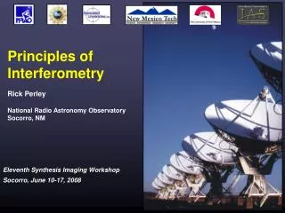
Fundamentals of Radio Interferometry. Rick Perley , NRAO/Socorro. Topics. Why Interferometry ? Groundwork: Brightness, Flux density, Power, Sensors, Antennas, and more … The Quasi-Monochromatic, Stationary, Radio-Frequency, Single Polarization Interferometer

E N D
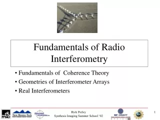
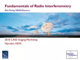
Fundamentals of Radio Interferometry Rick Perley, NRAO/Socorro
Topics • Why Interferometry? • Groundwork: Brightness, Flux density, Power, Sensors, Antennas, and more … • The Quasi-Monochromatic, Stationary, Radio-Frequency, Single Polarization Interferometer • Complex Visibility and its relation to Brightness
Why Interferometry? • Radio telescopes coherently sum electric fields over an aperture of size D. • For this, diffraction theory applies – the angular resolution is: • In ‘practical’ units: • To obtain 1 arcsecond resolution at a wavelength of 21 cm, we require an aperture of ~42 km! • Can we synthesize an aperture of that size with pairs of antennas? • The methodology of synthesizing a continuous aperture through summations of separated pairs of antennas is called ‘aperture synthesis’. 2008 ATNF Synthesis Imaging School
Spectral Flux Density and Brightness • Our Goal: To measure the characteristics of celestial emission from a given direction s, at a given frequency n, at a given time t. • In other words: We want a map, or image, of the emission. • Terminology/Definitions: The quantity we seek is called the brightness (or specific intensity): It is denoted here by I(s,n,t), and expressed in units of: watt/(m2 Hz ster). • It is the power received, per unit solid angle from direction s, per unit collecting area, per unit frequency at frequency n. • Do not confuse I with Flux Density, S -- the integral of the brightness over a given solid angle: • The units of Sare: watt/(m2 Hz) • Note: 1 Jy = 10-26 watt/(m2 Hz). Twelfth Synthesis Imaging Workshop
An Example – Cygnus A • I show below an image of Cygnus A at a frequency of 4995 MHz. • The units of the brightness are Jy/beam, with 1 beam = 0.16 arcsec2 • The peak is 2.6 Jy/beam, which equates to 6.5 x 10⁻¹⁵ watt/(m2 Hz ster) • The flux density of the source is 370 Jy = 3.7 x 10⁻²⁴ watt/(m2 Hz) Twelfth Synthesis Imaging Workshop
Intensity and Power. dW • Imagine a distant source of emission, described by brightness I(n,s) where s is a unit direction vector. • Power from this emission is intercepted by a collector (`sensor’) of area A(n,s). • The power, P (watts) from a small solid angle dW, within a small frequency window dn, is • The total power received is an integral over frequency and angle, accounting for variations in the responses. Solid Angle Sensor Area Filter width Power collected s A dn P Twelfth Synthesis Imaging Workshop
The Role of the Sensor • Coherent interferometry is based on the ability to correlate the electric fields measured at spatially separated locations. • To do this (without mirrors) requires conversion of the electric field E(r,n,t) at some place to a voltage V(n,t) which can be conveyed to a central location for processing. • For our purpose, the sensor (a.k.a. ‘antenna’) is simply a device which senses the electric field at some place and converts this to a voltage which faithfully retains the amplitudes and phases of the electric fields. • One can imagine two kinds of ideal sensors: • An ‘all-sky’ sensor: All incoming electric fields, from all directions, are uniformly summed. • The ‘limited-field-of-view’ sensor: Only the fields from a given direction and solid angle (field of view) are collected and conveyed. • Sadly – neither of these is possible. 2008 ATNF Synthesis Imaging School
Quasi-Monochromatic Radiation • Analysis is simplest if the fields are perfectly monochromatic. • This is not possible – a perfectly monochromatic electric field would both have no power (Dn = 0), and would last forever! • So we consider instead ‘quasi-monochromatic’ radiation, where the bandwidth dn is finite, but very small compared to the frequency: dn << n • Consider then the electric fields from a small sold angle dWabout some direction s, within some small bandwidth dn, at frequency n. • We can write the temporal dependence of this field as: • The amplitude and phase remains unchanged to a time duration of order dt ~1/dn, after which new values of E and f are needed. 2008 ATNF Synthesis Imaging School
Simplifying Assumptions • We now consider the most basic interferometer, and seek a relation between the characteristics of the product of the voltages from two separated antennas and the distribution of the brightness of the originating source emission. • To establish the basic relations, the following simplifications are introduced: • Fixed in space – no rotation or motion • Quasi-monochromatic • No frequency conversions (an ‘RF interferometer’) • Single polarization • No propagation distortions (no ionosphere, atmosphere …) • Idealized electronics (perfectly linear, perfectly uniform in frequency and direction, perfectly identical for both elements, no added noise, …)
The Stationary, Quasi-Monochromatic Radio-Frequency Interferometer s s Geometric Time Delay b.s b The path lengths from sensors to multiplier are assumed equal! X multiply average Unchanging Rapidly varying, with zero mean
Pictorial Example: Signals In Phase 2 GHz Frequency, with voltages in phase: b.s = nl, ortg =n/n • Antenna 1 Voltage • Antenna 2 Voltage • Product Voltage • Average 2008 ATNF Synthesis Imaging School
Pictorial Example: Signals in Quad Phase 2 GHz Frequency, with voltages in quadrature phase: b.s=(n +/- ¼)l, tg= (4n +/- 1)/4n • Antenna 1 Voltage • Antenna 2 Voltage • Product Voltage • Average 2008 ATNF Synthesis Imaging School
Pictorial Example: Signals out of Phase 2 GHz Frequency, with voltages out of phase: b.s=(n +/- ½)ltg= (2n +/- 1)/2n • Antenna 1 Voltage • Antenna 2 Voltage • Product Voltage • Average 2008 ATNF Synthesis Imaging School
Some General Comments • The averaged product RCis dependent on the received power, P = E2/2 and geometric delay, tg, and hence on the baseline orientation and source direction: • Note that RCis not a a function of: • The time of the observation -- provided the source itself is not variable! • The location of the baseline -- provided the emission is in the far-field. • The actual phase of the incoming signal – the distance of the source does not matter, provided it is in the far-field. • The strength of the product is dependent on the antenna areas and electronic gains – but these factors can be calibrated for. 2008 ATNF Synthesis Imaging School
Pictorial Illustrations • To illustrate the response, expand the dot product in one dimension: • Here, u = b/lis the baseline length in wavelengths, andqis the angle w.r.t. the plane perpendicular to the baseline. • is the direction cosine • Consider the response Rc, as a function of angle, for two different baselines with u = 10, and u = 25 wavelengths: s q a b 2008 ATNF Synthesis Imaging School
Whole-Sky Response -10 -8 -5 -3 0 2 7 10 5 9 • Top: u = 10 There are 20 whole fringes over the hemisphere. • Bottom: u = 25 There are 50 whole fringes over the hemisphere -25 25
From an Angular Perspective q 0 3 Top Panel: The absolute value of the response for u = 10, as a function of angle. The ‘lobes’ of the response pattern alternate in sign. Bottom Panel: The same, but for u = 25. Angular separation between lobes (of the same sign) is dq ~ 1/u = l/b radians. 5 7 + - + 9 - + 10
Hemispheric Pattern • The preceding plot is a meridional cut through the hemisphere, oriented along the baseline vector. • In the two-dimensional space, the fringe pattern consists of a series of coaxial cones, oriented along the baseline vector. • The figure is a two-dimensional representation when u = 4. • As viewed along the baseline vector, the fringes show a ‘bulls-eye’ pattern – concentric circles. Twelfth Synthesis Imaging Workshop
The Effect of the Sensor • The patterns shown presume the sensor has isotropic response. • This is a convenient assumption, but (sadly, in some cases) doesn’t represent reality. • Real sensors impose their own patterns, which modulate the amplitude and phase, of the output. • Large sensors (a.k.a. ‘antennas’) have very high directivity --very useful for some applications.
The Effect of Sensor Patterns • Sensors (or antennas) are not isotropic, and have their own responses. • Top Panel: The interferometer pattern with a cos(q)-like sensor response. • Bottom Panel: A multiple-wavelength aperture antenna has a narrow beam, but also sidelobes.
The Response from an Extended Source • The response from an extended source is obtained by summing the responses at each antenna to all the emission over the sky, multiplying the two, and averaging: • The averaging and integrals can be interchanged and, providing the emission is spatially incoherent, we get • This expression links what we want – the source brightness on the sky, In(s), – to something we can measure - RC, the interferometer response. • Can we recover In(s) from observations of RC? 2008 ATNF Synthesis Imaging School
A Schematic Illustration in 2-D • The correlator can be thought of ‘casting’ a cosinusoidal coherence pattern, of angular scale~l/b radians, onto the sky. • The correlator multiplies the source brightness by this coherence pattern, and integrates (sums) the result over the sky. l/b • Orientation set by baseline geometry. • Fringe separation set by (projected) baseline length and wavelength. • Long baseline gives close-packed fringes • Short baseline gives widely-separated fringes • Physical location of baseline unimportant, provided source is in the far field. l/b rad. Source brightness - + - + - + - Fringe Sign
Odd and Even Functions • Any real function, I(x,y),can be expressed as the sum of two real functions which have specific symmetries: An even part: An odd part: IE IO I IE IO I = + 2008 ATNF Synthesis Imaging School
But One Correlator is Not Enough! • The correlator response, Rc: is not enough to recover the correct brightness. Why? • Suppose that the source of emission has a component with odd symmetry: Io(s) = -Io(-s) • Since the cosine fringe pattern is even, the response of our interferometer to the odd brightness distribution is 0! • Hence, we need more information if we are to completely recover the source brightness. 2008 ATNF Synthesis Imaging School
Why Two Correlations are Needed • The integration of the cosine response, Rc, over the source brightness is sensitive to only the even part of the brightness: since the integral of an odd function (IO) with an even function (cos x) is zero. • To recover the ‘odd’ part of the intensity, IO, we need an ‘odd’ fringe pattern. Let us replace the ‘cos’ with ‘sin’ in the integral since the integral of an even times an odd function is zero. • To obtain this necessary component, we must make a ‘sine’ pattern.
Making a SIN Correlator • We generate the ‘sine’ pattern by inserting a 90 degree phase shift in one of the signal paths. s s b.s b A Sensor X 90o multiply average
Define the Complex Visibility • We now DEFINE a complex function, the complex visibility, V, from the two independent (real) correlator outputs RC and RS: where • This gives us a beautiful and useful relationship between the source brightness, and the response of an interferometer: • Under some circumstances, this is a 2-D Fourier transform, giving us a well established way to recover I(s) from V(b).
The Complex Correlator and Complex Notation • A correlator which produces both ‘Real’ and ‘Imaginary’ parts – or the Cosine and Sine fringes, is called a ‘Complex Correlator’ • For a complex correlator, think of two independent sets of projected sinusoids, 90 degrees apart on the sky. • In our scenario, both components are necessary, because we have assumed there is no motion – the ‘fringes’ are fixed on the source emission, which is itself stationary. • The complex output of the complex correlator also means we can use complex analysis throughout: Let: • Then:
Picturing the Visibility • The source brightness is Gaussian, shown in black. • The interferometer ‘fringes’ are in red. • The visibility is the integral of the product – the net dark green area. RC RS Long Baseline Long Baseline Short Baseline Short Baseline
Examples of 1-Dimensional Visibilities • Simple pictures are easy to make illustrating 1-dimensional visibilities. • Brightness Distribution Visibility Function • Unresolved Doubles • Uniform • Central Peaked Twelfth Synthesis Imaging Workshop
More Examples • Simple pictures are easy to make illustrating 1-dimensional visibilities. • Brightness Distribution Visibility Function • Resolved Double • Resolved Double • Central Peaked Double Twelfth Synthesis Imaging Workshop
Basic Characteristics of the Visibility • For a zero-spacing interferometer, we get the ‘single-dish’ (total-power) response. • As the baseline gets longer, the visibility amplitude will in general decline. • When the visibility is close to zero, the source is said to be ‘resolved out’. • Interchanging antennas in a baseline causes the phase to be negated – the visibility of the ‘reversed baseline’ is the complex conjugate of the original. • Mathematically, the visibility is Hermitian, because the brightness is a real function.
Some Comments on Visibilities • The Visibility is a unique function of the source brightness. • The two functions are related through a Fourier transform. • An interferometer, at any one time, makes one measure of the visibility, at baseline coordinate (u,v). • Sufficient knowledge of the visibility function (as derived from an interferometer) will provide us a reasonable estimate of the source brightness. • How many is ‘sufficient’, and how good is ‘reasonable’? • These simple questions do not have easy answers…