Download
1 / 51
520 likes | 845 Vues
Fundamentals of Radio Interferometry Rick Perley Outline Antennas – Our Connection to the Universe The Monochromatic, Stationary Interferometer The Relation between Brightness and Visibility Coordinate Systems Making Images The Consequences of Finite Bandwidth

E N D
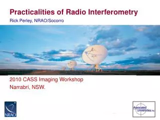
Fundamentals of Radio Interferometry Rick Perley
Outline • Antennas – Our Connection to the Universe • The Monochromatic, Stationary Interferometer • The Relation between Brightness and Visibility • Coordinate Systems • Making Images • The Consequences of Finite Bandwidth • Adding Time Delay and Motion • Heterodyning • The Consequences of Finite Time Averaging R. Perley, Synthesis Imaging Summer School, 15-22 June 2004
Telescopes – our eyes (ears?) on the Universe • Nearly all we know of our universe is through observations of electromagnetic radiation. • The purpose of an astronomical telescope is to determine the characteristics of this emission: • Angular distribution • Frequency distribution • Polarization characteristics • Temporal characteristics • Telescopes are sophisticated, but imperfect devices, and proper use requires an understanding of their capabilities and limitations. R. Perley, Synthesis Imaging Summer School, 15-22 June 2004
Antennas – the Single Dish • The simplest radio telescope (other than elemental devices such as a dipole or horn) is a parabolic reflector – a ‘single dish’. • The detailed characteristics of single dishes are covered in the next lecture. Here, we comment only on four important characteristics, and on a simple explanation for these: • They have a directional gain. • They have an angular resolution given by: q ~ l/D. • They have ‘sidelobes’ – finite response at large angles. • Their angular response contains no sharp edges. • A basic understanding of the origin of these characteristics will aid in understanding the functioning of an interferometer. R. Perley, Synthesis Imaging Summer School, 15-22 June 2004
The Standard Parabolic Antenna Response R. Perley, Synthesis Imaging Summer School, 15-22 June 2004
Beam Pattern Origin An antenna’s response is a result of incoherent phase summation at the focus. First null will occur at the angle where the extra distance for a wave at center of antenna is in anti-phase with that from edge. On-axis incidence Off-axis incidence R. Perley, Synthesis Imaging Summer School, 15-22 June 2004
Getting Better Resolution • The 25-meter aperture of a VLA antenna provides insufficient resolution for modern astronomy. • 30 arcminutes at 1.4 GHz, when we want 1 arcsecond or better! • The trivial solution of building a bigger telescope is not practical. 1 arcsecond resolution at l = 20 cm requires a 40 kilometer aperture. • The world’s largest fully steerable antenna (operated by the NRAO at Green Bank, WV) has an aperture of only 100 meters Þ 4 times better resolution than a VLA antenna. • As this is not practical, we must consider a means of synthesizing the equivalent aperture, through combinations of elements. • This method, termed ‘aperture synthesis’, was developed in the 1950s in England and Australia. Martin Ryle (University of Cambridge) earned a Nobel Prize for his contributions. R. Perley, Synthesis Imaging Summer School, 15-22 June 2004
Aperture Synthesis – Basic Concept If the source emission is unchanging, there is no need to collect all of the incoming rays at one time. One could imagine sequentially combining pairs of signals. If we break the aperture into N sub- apertures, there will be N(N-1)/2 pairs to combine. This approach is the basis of aperture synthesis. R. Perley, Synthesis Imaging Summer School, 15-22 June 2004
The Stationary, Monochromatic Interferometer A small (but finite) frequency width, and no motion. Consider radiation from a small solid angle dW, from direction s. s s b An antenna X multiply average
Examples of the Signal Multiplications The two input signals are shown in red and blue. The desired coherence is the average of the product (black trace) In Phase: tg =nl/c Quadrature Phase: tg=(2n+1)l/4c Anti-Phase: tg= (2n+1)l/2c R. Perley, Synthesis Imaging Summer School, 15-22 June 2004
Signal Multiplication, cont. • The averaged signal is independent of the time t, but is dependent on the lag, tg – a function of direction, and hence on the distribution of the brightness. • In this expression, we use ‘V’ to denote the voltage of the signal. This depends upon the source intensity by: so the term V1V2 is proportional to source intensity, In. (measured in Watts.m-2.Hz-2.ster-2). • The strength of the product is also dependent on the antenna areas and electronic gains – but these factors can be calibrated for. • To determine the dependence of the response over an extended object, we integrate over solid angle. R. Perley, Synthesis Imaging Summer School, 15-22 June 2004
The ‘Cosine’ Correlator Response • The response from an extended source is obtained by integrating the response over the solid angle of the sky: where I have ignored (for now) any frequency dependence. Key point: the vector s is a function of direction, so the phase in the cosine is dependent on the angle of arrival. This expression links what we want – the source brightness on the sky) (In(s)) – to something we can measure (RC, the interferometer response). R. Perley, Synthesis Imaging Summer School, 15-22 June 2004
A Schematic Illustration The COS correlator can be thought of ‘casting’ a sinusoidal fringe pattern, of angular scalel/B radians, onto the sky. The correlator multiplies the source brightness by this wave pattern, and integrates (adds) the result over the sky. Orientation set by baseline geometry. Fringe separation set by baseline length and wavelength. l/B rad. Source brightness - + - + - + - Fringe Sign R. Perley, Synthesis Imaging Summer School, 15-22 June 2004
Odd and Even Functions • But the measured quantity, Rc, is insufficient – it is only sensitive to the ‘even’ part of the brightness, IE(s). • Any real function, I, can be expressed as the sum of two real functions which have specific symmetries: An even part: IE(x,y) = (I(x,y) + I(-x,-y))/2 = IE(-x,-y) An odd part: IO(x,y) = (I(x,y) – I(-x,-y))/2 = -IO(-x,-y) IE IO I = + R. Perley, Synthesis Imaging Summer School, 15-22 June 2004
Recovering the ‘Odd’ Part: The SIN Correlator The integration of the cosine response, Rc, over the source brightness is sensitive to only the even part of the brightness: since the integral of an odd function (IO) with an even function (cos x) is zero. To recover the ‘odd’ part of the intensity, IO, we need an ‘odd’ coherence pattern. Let us replace the ‘cos’ with ‘sin’ in the integral: since the integral of an even times an odd function is zero. To obtain this necessary component, we must make a ‘sine’ pattern. R. Perley, Synthesis Imaging Summer School, 15-22 June 2004
Making a SIN Correlator • We generate the ‘sine’ pattern by inserting a 90 degree phase shift in one of the signal paths. s s b An antenna X 90o multiply average
Define the Complex Visibility We now DEFINE a complex function, V, to be the complex sum of the two independent correlator outputs: where This gives us a beautiful and useful relationship between the source brightness, and the response of an interferometer: Although it may not be obvious (yet), this expression can be inverted to recover I(s) from V(b). R. Perley, Synthesis Imaging Summer School, 15-22 June 2004
Picturing the Visibility • The intensity, In, is in black, the ‘fringes’ in red. The visibility is the net dark green area. RC RS Long Baseline Short Baseline
Comments on the Visibility • The Visibility is a function of the source structure and the interferometer baseline. • The Visibility is NOT a function of the absolute position of the antennas (provided the emission is time-invariant, and is located in the far field). • The Visibility is Hermitian: V(u,v) = V*(-u,-v). This is a consequence of the intensity being a real quantity. • There is a unique relation between any source brightness function, and the visibility function. • Each observation of the source with a given baseline length provides one measure of the visibility. • Sufficient knowledge of the visibility function (as derived from an interferometer) will provide us a reasonable estimate of the source brightness. R. Perley, Synthesis Imaging Summer School, 15-22 June 2004
Examples of Visibility Functions • Top row: 1-dimensional even brightness distributions. • Bottom row: The corresponding real, even, visibility functions. R. Perley, Synthesis Imaging Summer School, 15-22 June 2004
Geometry – the perfect, and not-so-perfect To give better understanding, we now specify the geometry. Case A: A 2-dimensional measurement plane. Let us imagine the measurements of Vn(b) to be taken entirely on a plane. Then a considerable simplification occurs if we arrange the coordinate system so one axis is normal to this plane. Let (u,v,w) be the coordinate axes, with w normal to the plane. All distances are measured in wavelengths. Then, the components of the unit direction vector, s, are: and R. Perley, Synthesis Imaging Summer School, 15-22 June 2004
Direction Cosines w The unit direction vectors is defined by its projections on the (u,v,w) axes. These components are called the Direction Cosines. s n g b a v m l b u The baseline vectorbis specified by its coordinates (u,v,w) (measured in wavelengths). R. Perley, Synthesis Imaging Summer School, 15-22 June 2004
The 2-d Fourier Transform Relation Then,nb.s/c = ul + vm + wn = ul + vm, from which we find, which is a2-dimensional Fourier transformbetween the projected brightness: and the spatial coherence function (visibility):Vn(u,v). And we can now rely on a century of effort by mathematicians on how to invert this equation, and how much information we need to obtain an image of sufficient quality. Formally, With enough measures of V, we can derive I. R. Perley, Synthesis Imaging Summer School, 15-22 June 2004
Interferometers with 2-d Geometry • Which interferometers can use this special geometry? a) Those whose baselines, over time, lie on a plane (any plane). All E-W interferometers are in this group. For these, the w-coordinate points to the NCP. • WSRT (Westerbork Synthesis Radio Telescope) • AT (Australia Telescope) • Cambridge 5km telescope (almost). b) Any coplanar array, at a single instance of time. • VLA or GMRTin snapshot (single short observation) mode. • What's the ‘downside’ of this geometry? • Full resolution is obtained only for observations that are in the w-direction. Observations at other directions lose resolution. • E-W interferometers have no N-S resolution for observations at the celestial equator!!! • A VLA snapshot of a source at the zenith will have no ‘vertical’ resolution for objects on the horizon. R. Perley, Synthesis Imaging Summer School, 15-22 June 2004
3-d Interferometers Case B: A 3-dimensional measurement volume: • But what if the interferometer does not measure the coherence function within a plane, but rather does it through a volume? In this case, we adopt a slightly different coordinate system. First we write out the full expression: (Note that this is not a 3-D Fourier Transform). • Then, orient the coordinate system so that the w-axis points to the center of the region of interest, (u points east and v north) and make use of the small angle approximation: where q is the polar angle from the center of the image. The w-component is the ‘delay distance’ of the baseline. R. Perley, Synthesis Imaging Summer School, 15-22 June 2004
VLA Coordinate System w points to the source, u towards the east, and v towards the NCP. The direction cosines l and m then increase to the east and north, respectively. w s0 s0 b v R. Perley, Synthesis Imaging Summer School, 15-22 June 2004
3-d to 2-d The quadratic term in the phase can be neglected if it is much less than unity: Or, in other words, if the maximum angle from the center is: (angles in radians!) then the relation between the Intensity and the Visibility again becomes a 2-dimensional Fourier transform: R. Perley, Synthesis Imaging Summer School, 15-22 June 2004
3-d to 2-d where the modified visibility is defined as: and is, in fact, the visibility we would have measured, had we been able to put the baseline on the w = 0 plane. • This coordinate system, coupled with the small-angle approximation, allows us to use two-dimensional transforms for any interferometer array. • How do we make images when the small-angle approximation breaks down? That's a longer story, for another day. (Short answer: we know how to do this, and it takes a lot more computing). R. Perley, Synthesis Imaging Summer School, 15-22 June 2004
Making Images We have shown that under certain (and attainable) assumptions about electronic linearity and narrow bandwidth, a complex interferometer measures the visibility, or complex coherence: (u,v) are the projected baseline coordinates, measured in wavelengths, on a plane oriented facing the phase center, and (l,m) are the sines of the angles between the phase center and the emission, in the EW and NS directions, respectively. R. Perley, Synthesis Imaging Summer School, 15-22 June 2004
Making Images This is a Fourier transform relation, and it can be in general be solved, to give: This relationship presumes knowledge of V(u,v) for all values of u and v. In fact, we have a finite number, N, measures of the visibility, so to obtain an image, the integrals are replaced with a sum: If we have Nv visibilities, and Nm cells in the image, we have ~NvNm calculations to perform – a number that can exceed 1012! R. Perley, Synthesis Imaging Summer School, 15-22 June 2004
But Images are Real • The sum on the last page is in general complex, while the sky brightness is real. What’s wrong? • In fact, each measured visibility represents two visibilities, since V(-u,-v) = V*(u,v). • This is because interchanging two antennas leaves Rc unchanged, but changes the sign of Rs. • Mathematically, as the sky is real, the visibility must be Hermitian. • So we can modify the sum to read: R. Perley, Synthesis Imaging Summer School, 15-22 June 2004
Interpretation • The cosine represents a two-dimensional sinusoidal function in the image, with unit amplitude, and orientation given by: a = tan-1(u/v). • The cosinusoidal sea on the image plane is multiplied by the visibility amplitude A, and a shifted by the visibility phase fn. • Each individual measurement adds a (shifted and amplified) cosinusoid to the image. • The basic (raw, or dirty) map is the result of this summation process. • The actual process, including the use of FFTs, is covered in the ‘imaging’ lecture. R. Perley, Synthesis Imaging Summer School, 15-22 June 2004
A simple example The rectangle below represents a piece of sky. The solid red lines are the maxima of the sinusoids, the dashed lines their minima. Two visibilities are shown, each with phase zero. m + a l - + - + R. Perley, Synthesis Imaging Summer School, 15-22 June 2004
1-d Example: Point-Source For a unit point source, all visibility amplitudes are 1 Jy, and all phases are zero. The lower panel shows the response when visibilities from 21 equally-spaced baselines are added. The individual visibilities are shown in the top panel. Their (incremental) sums are shown in the lower panel. R. Perley, Synthesis Imaging Summer School, 15-22 June 2004
Example 2: Square Source • For a centered square object, the visibility amplitudes decline with increasing baseline, and the phases are all zero or 180. • Again, 21 baselines are included. R. Perley, Synthesis Imaging Summer School, 15-22 June 2004
The Effect of Bandwidth. Real interferometers must accept a range of frequencies (amongst other things, there is no power in an infinitesimal bandwidth)! So we now consider the response of our interferometer over frequency. To do this, we first define the frequency response functions, G(n), as the amplitude and phase variation of the signals paths over frequency. Then integrate: Dn G n n0 R. Perley, Synthesis Imaging Summer School, 15-22 June 2004
The Effect of Bandwidth. If the source intensity does not vary over frequency width, we get where I have assumed the G(n) are square, real, and of widthDn. The frequencyn0 is the mean frequency within the bandwidth. The fringe attenuation function, sinc(x), is defined as: for x << 1 R. Perley, Synthesis Imaging Summer School, 15-22 June 2004
The Bandwidth/FOV limit This shows that the source emission is attenuated by the function sinc(x), known as the ‘fringe-washing’ function. Noting thattg ~ (B/c) sin(q) ~Bq/ln ~ (q/qres)/n, we see that the attenuation is small when The ratioDn/nis the fractional bandwidth. The ratioq/qresis the source offset in units of the fringe separation,l/B. In words, this says that the attenuation is small if the fractional bandwidth times the angular offset in resolution units is less than unity. Significant attenuation of the measured visibility is to be expected if the source offset is comparable to the interferometer resolution divided by the fractional bandwidth. R. Perley, Synthesis Imaging Summer School, 15-22 June 2004
Bandwidth Effect Example Finite Bandwidth causes loss of coherence at large angles, because the amplitude of the interferometer fringes are reduced with increasing angle from the delay center. R. Perley, Synthesis Imaging Summer School, 15-22 June 2004
Avoiding Bandwidth Losses • The trivial solution is to avoid observing large objects! (Not helpful). • Although there are computational methods which allow recovery of the lost amplitude, the loss in SNR is unavoidable. • The simple solution is to observe with a small bandwidth. But this causes loss of sensitivity. • So, the best (but not cheapest!) solution is to observe with LOTS of narrow channels. • Modern correlators will provide tens to hundreds of thousands of channels of appropriate width. R. Perley, Synthesis Imaging Summer School, 15-22 June 2004
Adding Time Delay • Another important consequence of observing with a finite bandwidth is that the sensitivity of the interferometer is not uniform over the sky. • The current analysis, when applies to a finite bandwidth interferometer, shows that only sources on a plane orthogonal to the interferometer baseline will be observed with full coherence. • How can we recover the proper visibility for sources far from this plane? • Add time delay to shift the maximum of the ‘sinc’ pattern to the direction of the source. R. Perley, Synthesis Imaging Summer School, 15-22 June 2004
The Stationary, Radio-Frequency Interferometerwith inserted time delay s0 s0 s s S0 = reference direction S = general direction tg b An antenna X t0 R. Perley, Synthesis Imaging Summer School, 15-22 June 2004
Coordinates • It should be clear from inspection that the results of the last section are reproduced, with the ‘fringes’ and the bandwidth delay pattern, how centered about the direction defined byt-tg= 0. The unattenuated field of view is as before: Dq/qres< n/Dn • Remembering the coordinate system discussed earlier, where the w axis points to the reference center (s0), assuming the introduced delay is appropriate for this center, and that the bandwidth losses are negligible, we have: R. Perley, Synthesis Imaging Summer School, 15-22 June 2004
Extension to a Moving Source • Inserting these, we obtain: • The third term in the exponential is generally very small, and can be ignored in most cases, as discussed before. • The extension to a moving source (or, more usually, to an interferometer located on a rotating object) is elementary – the delay termtchanges with time, so as to keep the peak of the fringe-washing function on the center of the region of interest. • Also note that for a point object at the tracking center (l = m = 0), the phase is zero. This is because the added delay has exactly matched the phase lag of the radiation on the lagged antenna. R. Perley, Synthesis Imaging Summer School, 15-22 June 2004
Consequence of IF Conversion • This would be the end of the story (so far as the fundamentals are concerned) if all the internal electronics of an interferometer would work at the observing frequency (often called the ‘radio frequency’, or RF). • Unfortunately, this cannot be done in general, as high frequency components are much more expensive, and generally perform more poorly, than low frequency components. • Thus, nearly all radio interferometers use ‘down-conversion’ to translate the radio frequency information from the ‘RF’, to a lower frequency band, called the ‘IF’ in the jargon of our trade. • For signals in the radio-frequency part of the spectrum, this can be done with almost no loss of information. But there is an important side-effect from this operation, which we now review. R. Perley, Synthesis Imaging Summer School, 15-22 June 2004
Downconversion tg cos(wRFt) wLO X fLO X Multiplier Local Oscillator Phase Shifter cos(wIFt+fLO) t (wRF=wLO+wIF) Complex Correlator X cos(wIFt-wIFt+f) cos(wIFt-wRFtg) R. Perley, Synthesis Imaging Summer School, 15-22 June 2004
Phase Addition • We want the phase of this output to be zero for emission from the reference direction:tg=t0. • We also want to maximize the coherence from this same direction:t = t0. • We get both if we set: The reason this is necessary is that the delay,t0, has been added in the IF portion of the signal path, rather than at the frequency at which the delay actually occurs. Thus, the physical delay needed to maintain broad-band coherence is present, but because it is added at the ‘wrong’ frequency, an incorrect phase has been inserted, which must be corrected by addition of the ‘missing’ phase in the LO portion. R. Perley, Synthesis Imaging Summer School, 15-22 June 2004
Time-Averaging Loss • We have assumed everywhere that the values of the visibility are obtained ‘instantaneously’. This is of course not reasonable, for we must average over a finite time interval. • The time averaging, if continued too long, will cause a loss of measured coherence which is quite analogous to bandwidth smearing. • The fringe-tracking interferometer keeps the phase constant for emission from the phase-tracking center. However, for any other position, the phase of a point of emission changes in time. The relation is: whereqis the source offset from the phase-tracking center. R. Perley, Synthesis Imaging Summer School, 15-22 June 2004
Time-Smearing Loss • Simple derivation of fringe frequency: • Light blue area is antenna primary beam on the sky. • Fringes (black lines) rotate about the center at rate we. • Time taken for a fringe to rotate by l/B at angular distance qis: t = (l/B)/weq> D/(weB) • Fringe frequency is then nf = weB/D we q l/B l/D R. Perley, Synthesis Imaging Summer School, 15-22 June 2004
Time-averaging Loss • The net visibility obtained after an integration time, t, is found by integration: • As with bandwidth loss, the condition for minimal time loss is that the integration time be much less than the inverse fringe frequency: • For VLA in A-configuration, t << 10 seconds R. Perley, Synthesis Imaging Summer School, 15-22 June 2004