Download
1 / 35
350 likes | 380 Vues
Explore the basics of radio interferometry and coherence theory in Rick Perley's Synthesis Imaging Summer School '02, illustrating how electromagnetic waves from distant sources are measured and used to study celestial phenomena.

E N D
Fundamentals of Radio Interferometry Fundamentals of Coherence Theory Geometries of Interferometer Arrays Real Interferometers Rick Perley Synthesis Imaging Summer School ‘02
A long time ago, in a galaxy far, far away … An electron was moved. This action caused an electromagnetic wave to be launched, which then propagated away, obeying the well-known Maxwell’s equations. At a later time, at another locale, this EM wave, and many others from all the other electrons in the universe, arrived at a sensing device (a.k.a. ‘antenna’). The superposition of all these fields creates an electric current in the antenna, which (thanks to very clever engineers) we can measure, and which gives us information about the electric field. What can we learn about the radiating source from such measures? Rick Perley Synthesis Imaging Summer School ‘02
Let us denote the coordinates of our electron by: (R, t), and the vector electric field by: E(R,t). The location of the ‘antenna’ is denoted by r. It is useful to think of these fields in terms of their spectral content. Imagine the voltage waveform going into a large filter bank, which decomposes the time-ordered field into its mono-chromatic components of the electric field, En(R). Because the mono-chromatic components of the field from the far-reaches of the universe add linearly, we can express the electric field at location r by: Where Pn(R,r) is the propagator, and describes how the fields at R influence those at r. Rick Perley Synthesis Imaging Summer School ‘02
An emitting electron (one of many) The ‘celestial sphere’ R R0 An observer r Rick Perley Synthesis Imaging Summer School ‘02
At this point we introduce simplifying assumptions: • Scalar fields: We consider a single scalar component of the vector field. The vector field E becomes a scalar component E, and the propagator Pn(R,r) reduces from a tensor to a scalar. • The origin of the emission is at a great distance, and there is no hope of ‘resolving’ the depth. We can then consider the emission to originate from a common distance, |R0| -- and with an equivalent electric field En(R0) • Space within this celestial sphere is empty. In this case, the propagator is particularly simple: • which simply says that the phase is retarded by 2pn|R-r|/c radians, and the amplitude diminished by a factor 1/|R-r|. Rick Perley Synthesis Imaging Summer School ‘02
We then have, for the monochromatic field component at our sampling point: Note that the integration over volume has been replaced with one of the equivalent field over the celestial surface. So – what can we do with this? By itself, it is not particular useful – an amplitude and phase at a point in time. But a ‘comparison’ of these fields at two different locations might provide useful information. This comparison can be quantified by forming the complex product of these fields when measured at two places, and averaging. Define the spatial coherence function as: Rick Perley Synthesis Imaging Summer School ‘02
We can now insert our expression for the summed monochromatic field at locations r1 and r2, to obtain a general expression for the quantity Vn,. The resulting expression is very long -- see Equation 3-1 in the book. We then introduce our fourth – and very important – assumption: 4. The fields are spatially incoherent. That is, when This means there is no long-term phase relationship between emission from different points on the celestial sphere. This condition can be violated in some cases (scattering, illumination of a screen from a common source), so be careful! Rick Perley Synthesis Imaging Summer School ‘02
Using this condition, we find (see Chap. 1 of the book): • Now we introduce two important quantities: • The unit direction vector, s: • The specific intensity, In: • And replace the surface element dS with the elemental solid angle: • Remembering that |R0| >> |r|, we find: Rick Perley Synthesis Imaging Summer School ‘02
This beautiful relationship between the specific intensity, or brightness, In(s) (which is what we seek), and the spatial coherence function Vn(r1,r2) (which is what we must measure) is the foundation of aperture synthesis in radio astronomy. It looks like a Fourier Transform – and in the next section we look to see under what conditions it becomes one. A key point is that the spatial coherence function (‘visibility’) is only dependent upon the separation vector: r1 - r2. We commonly refer to this as the baseline: Rick Perley Synthesis Imaging Summer School ‘02
Geometry – the perfect, and not-so-perfect Case A: A 2-dimensional measurement plane. Let us imagine the measurements of Vn(r1,r2) to be taken entirely on a plane. Then a considerable simplification occurs if we arrange the coordinate system so one axis is normal to this plane. Let u, v, w be the rectangular components of the baseline vector, b, measured in units of the wavelength. Orient this reference system so w is normal to the plane on which the visibilities are measured. Then, in the same coordinate system, the unit direction vector, s, has components (the direction cosines) as follows: and Rick Perley Synthesis Imaging Summer School ‘02
w s g b a v u Rick Perley Synthesis Imaging Summer School ‘02
We then get: which is a 2-dimensional Fourier transform between the projected brightness: and the spatial coherence function (visibility): Vn(u,v). And we can now rely on a century of effort by mathematicians on how to invert this equation, and how much information we need to obtain an image of sufficient quality. Formally, With enough measures of V, we can derive I. Rick Perley Synthesis Imaging Summer School ‘02
Case B: A 3-dimensional measurement volume: But what if the interferometer does not measure the coherence function within a plane, but rather does it through a volume? In this case, we adopt a slightly different coordinate system. First we write out the full expression: (Note that this is not a 3-D Fourier Transform). Then, orient the coordinate system so that the w-axis points to the center of the region of interest, and make use of the small angle approximation: Rick Perley Synthesis Imaging Summer School ‘02
The quadratic term in the phase can be neglected if it is much less than unity: Or, in other words, if the maximum angle from the center is less than: then the relation between the Intensity and the Visibility again becomes a 2-dimension Fourier transform: Rick Perley Synthesis Imaging Summer School ‘02
Where the modified visibility is defined as: And is, in fact, the ‘true’ visibility, projected onto the w=0 plane, with the appropriate phase shift for the direction of the image center. I leave to you the rest of Chapter 1 in the book. It continues with the effects of discrete sampling, the effect of the antenna power reception pattern, some essentials of spectroscopy, and a discourse into polarimetry. We now go on to consider a ‘real’ interferometer, and learn how these complex coherence functions are actually measured. Rick Perley Synthesis Imaging Summer School ‘02
The Stationary, Radio-Frequency Interferometer The simplest possible interferometer is sketched below: s s b An antenna X Rick Perley Synthesis Imaging Summer School ‘02
In this expression, we use ‘A’ to denote the amplitude of the signal. In fact, the amplitude is a function of the antenna gain and cable losses (which we ignore here), and the intensity of the source of emission. The spectral intensity, or brightness, is defined as the power per unit area, per unit frequency width, per unit solid angle, from direction s, at frequency n. Thus, (ignoring the antenna’s gains and losses), the power available at the voltage multiplier becomes: The response from an extended source (or the entire sky) is obtained by integrating over the solid angle of the sky: Rick Perley Synthesis Imaging Summer School ‘02
This expression is close to what we are looking for. But because the cosine function is even, the integration over the sky of the correlator output will only be sensitive to the even part of the brightness distribution – it is insensitive to the ‘odd’ part. We can construct an interferometer which is sensitive to only the odd part of the brightness by building a 2nd multiplier, and inserting a 90 degree phase shift into one of the signal paths, prior to the multiplier. Then, a straightforward calculation shows the output of this correlator is: We now have two, independent numbers, each of which gives unique information about the sky brightness. We can then define a complex quantity – the complex visibility, by: Rick Perley Synthesis Imaging Summer School ‘02
This is the same expression we found earlier – allowing us to identify this complex function with the spatial coherence function. So the function we need to measure, in order to recover the brightness of a distant radio source (the intensity) is provided by a complex correlator, consisting of a ‘cosine’ and ‘sine’ multiplier. In this analysis, we have used real functions, then created the complex visibility by combining the cosine and sine outputs. This corresponds to what the interferometer does, but is clumsy analytically. A more powerful technique uses the ‘analytic signal’, which for this case consists of replacing cos(wt+j) with , then taking the complex product <V1V2*>. A demonstration that this leads (more cleanly) to the desired result I leave to the student! Rick Perley Synthesis Imaging Summer School ‘02
What’s going on here? How can we conveniently think of this? The COS correlator can be thought of ‘casting’ a sinuoisidal fringe pattern onto the sky. The correlator multiplies the source brightness by this wave pattern, and integrates (adds) the result over the sky. Fringe pattern cast on the source. Orientation set by baseline geometry Fringe separation set by baseline length. + - + - + - + - Fringe Sign The SIN correlator pattern is offset by ¼ wavelength. Rick Perley Synthesis Imaging Summer School ‘02
The more widely separated the ‘fringes’, the ‘more of the source’ is seen in one fringe lobe. Widely separated fringes are generated by short spacings – hence the total flux of the source is visible only when the fringe separation is much greater than the source extent. Conversely, the fine details of the source structure are only discernible when the fringe separation is comparable to the fine structure size and/or separation. To fully measure the source structure, a wide variety of baseline lengths and orientations is needed. One can build this up slowly with a single interferometer, or more quickly with a multi-telescope interferometer. Rick Perley Synthesis Imaging Summer School ‘02
Rick Perley Synthesis Imaging Summer School ‘02
Rick Perley Synthesis Imaging Summer School ‘02
The Effect of Bandwidth. Real interferometers must accept a range of frequencies (amongst other things, there is no power in an infinitesimal bandwidth)! So we now consider the response of our interferometer over frequency. To do this, we first define the frequency response functions, G(n), as the amplitude and phase variation of the signals paths over frequency. Inserting these, and taking the complex product, we get: Where I have left off the integration over angle for clarity. If the source intensity does not vary over frequency width, we get where I have assumed the bandpasses are square and of width Dn. Rick Perley Synthesis Imaging Summer School ‘02
The sinc function is defined as: when px << 1 This shows that the source emission is attenuated by the function sinc(x), known as the ‘fringe-washing’ function. Noting that tg ~ B/c sin(q) ~ Bq/ln ~ (q/qres)/n, we see that the attenuation is small when In words, this says that the attenuation is small if the fractional bandwidth times the angular offset in resolution units is less than unity. If the field of view is large, one must observe with narrow bandwidths, in order to measure a correct visibility. Rick Perley Synthesis Imaging Summer School ‘02
Rick Perley Synthesis Imaging Summer School ‘02
So far, the analysis has proceeded with the implicit assumption that the center of the image is stationary, and located straight up, perpendicular to the plane of the baseline. This is an unnecessary restriction, and I now go on to the more general case where the center of interest is not ‘straight up’, and is moving. In fact, this is an elementary addition to what we’ve already done. Since the effect of bandwidth is to restrict the region over which correct measures are made to a zone centered in the direction of zero time delay, it should be obvious that to observe in some other direction, we must add delay to move the unattenuated zone to the direction of interest. That is, we must add time delay to the ‘nearer’ side of the interferometer, to shift the unattenuated response to the direction of interest. Rick Perley Synthesis Imaging Summer School ‘02
The Stationary, Radio-Frequency Interferometer with inserted time delay s0 s0 s s b An antenna X t Rick Perley Synthesis Imaging Summer School ‘02
It should be clear from inspection that the results of the last section are reproduced, with the chromatic aberration now occurring about the direction defined by t – tg = 0. That is, the condition becomes: Dq/qres> n/Dn Remembering the coordinate system discussed earlier, where the w axis points to the reference center (s0), assuming the introduced delay is appropriate for this center, and that the bandwidth losses are negligible, we have: Rick Perley Synthesis Imaging Summer School ‘02
Inserting these, we obtain: This is the same relationship we derived in the earlier section. The extension to a moving source (or, more correctly, to an interferometer located on a rotating object) is elementary – the delay term t changes with time, so as to keep the peak of the fringe-washing function on the center of the region of interest. We will now complete our tour of elementary interferometers with a discussion of the effects of frequency downconversion. Rick Perley Synthesis Imaging Summer School ‘02
Ideally, all the internal electronics of an interferometer would work at the observing frequency (often called the ‘radio frequency’, or RF). Unfortunately, this cannot be done in general, as high frequency components are much more expensive, and generally perform more poorly, than low frequency components. Thus, nearly all radio interferometers use ‘downconversion’ to translate the radio frequency information to a lower frequency band. For signals in the radio-frequency part of the spectrum, this can be done with almost no loss of information. But there is an important side-effect from this operation, which we now quickly review. Rick Perley Synthesis Imaging Summer School ‘02
tg cos(wRFt) wLO X fLO X cos(wIFt+fLO) t (wRF=wLO+wIF) X cos(wIFt-wRFtg) cos(wIFt-wIFt+f) This is identical to the ‘RF’ interferometer, provided fLO = wLOt Rick Perley Synthesis Imaging Summer School ‘02
Thus, the frequency-conversion interferometer (which is getting quite close to the ‘real deal’, will provide the correct measure of the spatial coherence, provided that the phase of the LO (local oscillator) on one side is offset by: The reason this is necessary is that the delay, t, has been added in the IF portion of the signal path. Thus, the physical delay needed to maintain broad-band coherence is present, but because it is added at the ‘wrong’ (IF) frequency, rather than at the ‘right’ (RF) frequendy, an incorrect phase has been inserted. The necessary adjustment is that corresponding to the difference frequency (the LO). Rick Perley Synthesis Imaging Summer School ‘02
Some Concluding Remarks I have given here an approach which is based on the idea of a complex correlator – two identical, parallel multiplies with a 90 degree phase shift introduced in one. This leads quite naturally to the formation of a complex number, which is identified with the complex coherence function. But, a complex correlator is not necessary, if one can find another way to obtain the two independent quantities (Cos, Sin, or Real, Imaginary) needed. A single multiplier, on a moving (or rotating) platform will allow such a pair of measures – for the fringe pattern will then ‘move’ over the region of interest, and the sinusoidal output can be described with two parameters (e.g., amplitude and phase). Rick Perley Synthesis Imaging Summer School ‘02
This approach might seem attractive (fewer multipliers) until one considers the rate at which data must be logged. For an interferometer on the earth, the fringe frequency can be shown to be: Here, u is the E-W component of the baseline, and we is the angular rotation rate of the earth: 7.3 x 10⁻⁵ rad/sec. For interferometers whose baselines exceed thousands of wavelengths, this fringe frequency would require very fast (and completely unnecessary) data logging and analysis. The purpose of ‘stopping’ the fringes is to permit a data logging rate which is based on the differential motion of sources about the center of the field of interest. For the VLA in ‘A’ configuration, this is typically a few seconds. Rick Perley Synthesis Imaging Summer School ‘02