5. Echantillonnage Introduction

1. 5. Echantillonnage Introduction CONTINUE Echantillonnage  temps Quantification  amplitude xq(t) xe(t) DISCRETISATION Echantillonnage : les variations se déroulant dans un temps plus petit que Te ne peuvent pas être acquises

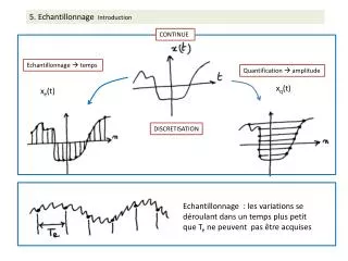
2. 5. Echantillonnage un exemple En NOIR continu : le signal original continu de période T (on dit signal sous-jacent) Points VERTs : le signal échantillonné avec pas de déformation Ronds ROUGES : le signal échantillonné « trop » lentement avec . On a l’impression que le signal est à plus basse fréquence qu’il ne l’est en réalité. On parle de « fréquence fantôme » ...

3. 5. Echantillonnage Principe L'échantillonnage consiste à discrétiser le temps des signaux analogiques continus. L'ensemble des échantillons prélevés constitue le signal échantillonné. Les échantillons sont prélevés à des intervalles de temps réguliers. La période entre deux échantillons consécutifs est appelée période d'échantillonnage et est notée Te. La fréquence d'échantillonnage est définie comme l'inverse de la période d'échantillonnage : Fe = 1/Te. Mathématiquement, l'opération « échantillonnage » s'écrit en utilisant la fonction peigne de Dirac telle que :

4. 5. Echantillonnage Spectre du signal échantillonné Soit x(t) un signal à spectre borné, on a : Le spectre Xe(f) s’obtient en périodisant le spectre initial X(f) sur l’axe des fréquences avec une période Fe. Un signal Te-échantillonné possède un spectre Fe-périodisé

5. 5. Echantillonnage Théorème de Shannon Fe > 2fmax : Le spectre Xe(t) contient le spectre de base X(f) sans déformation : Fe > 2fmax Fe < 2fmax :Le spectre de base est plus large, il y recouvrement et on ne retrouve plus X(f) dans Xe(f) : Théorème de Shannon : Pour qu’il n’y ait pas déformation du spectre  Fe > 2fmax

6. 5. Echantillonnage Filtrage anti-repliement Echantillonnage  périodisation du spectre  filtrage analogique passe-bas de fréquence de coupure Fe/2 le signal avant échantillonnage. Dans l’exemple ci-dessous, on échantillonne à 40 kHz un signal possédant une composante à 32 kHz. En rouge le spectre initial translaté d’une valeur Fe. Après reconstruction, le spectre contient une raie « fantôme » à 8 kHz !!!

7. Théorème de Shannon (I) Exécuter et étudier ce programme : t_fin=12e-2; t = 0:0.0001:t_fin; y = sin(2*pi*100*t); subplot(411), plot(t,y) hold on t = 0:0.0008:t_fin; y = sin(2*pi*100*t); subplot(411), plot(t,y,'or') t = 0:0.0001:t_fin; y = sin(2*pi*100*t); subplot(412), plot(t,y) hold on t = 0:0.00125:t_fin; y = sin(2*pi*100*t); subplot(412), plot(t,y,'or') t = 0:0.0001:t_fin; y = sin(2*pi*100*t); subplot(413), plot(t,y) hold on t = 0:0.00225:t_fin; y = sin(2*pi*100*t); subplot(413), plot(t,y,'or') t = 0:0.0001:t_fin; y = sin(2*pi*100*t); subplot(414), plot(t,y) hold on t = 0:0.0111:t_fin; y = sin(2*pi*100*t); subplot(414), plot(t,y,'-or') Quelle est la fréquence du signal y(t) ? Combien de périodes devrait on observer sur le domaine t [0, 0.12]. Est-ce le cas de la dernière courbe rouge ? Expliquer en termes de fréquences.

8. Théorème de Shannon (II) En reprenant les données de l’ exercice précèdent et en utilisant la fonction simul_TF, montrer qu’on a la propriété suivante pour un signal échantillonné :

9. Utilisation de la commande soundsc : Réaliser, étudier et commenter le programme suivant: Te=0.001; Fe=1/Te; t = 0:Te:1; y = sin(2*pi*80*t) + 2*sin(2*pi*160*t); yn = y + 0.5*randn(size(t)); plot(t(1:50),yn(1:50)) soundsc(y, Fe); disp('Taper sur la touche "Entrée" pour continuer'); pause; soundsc(yn,Fe); Ecouter le repliement 1/ Créer un vecteur temps t s’étendant de 0 à 2 secondes avec une fréquence d’échantillonnage Fe=5000 Hz. 2/ Créer le signal x(t) = f[sin(2*pi*f*t)] avec f=100, 200, 300, ..., 1000 Hz. Représenter x(t) et sa TF, X(f). Ecouter x(t) avec la fonction soundsc. 3/ Mêmes expériences avec Fe=2500 Hz et Fe=1750 Hz. Interpréter.

10. 5. Echantillonnage Reconstruction (I)

11. 5. Echantillonnage Reconstruction (II)