Multiscale Modelling
Multiscale Modelling. Mateusz Sitko. Faculty of Metals Engineering and Industrial Computer Science Department of Applied Computer Science and Modelling Kraków 11 -03-2014. Mateusz Sitko B5*607 msitko@agh.edu.pl consultation: Tuesday 1 3 :00 – 1 4 :00. Classes calendar. 2 reports:

Multiscale Modelling
E N D
Presentation Transcript
Multiscale Modelling Mateusz Sitko Faculty of Metals Engineering and Industrial Computer ScienceDepartment of Applied Computer Science and Modelling Kraków 11-03-2014
Mateusz Sitko B5*607 msitko@agh.edu.pl consultation: Tuesday 13:00 – 14:00
2 reports: • 1st – Grain growth algorithm modification (Cellular automata, Monte Carlo) • 2nd – Monte Carlo static recrystallization algorithm + grid infrastructure • Final degree will be positive if each report gets min 3.0 • 2 unexcused absences (remainder – medical leave)
CA method The main idea of the cellular automata technique is to divide a specific part of the material into one-, two-, or three-dimensional lattices of finite cells, where cells have clearly defined interaction rules between each other. Each cell in this space is called a cellular automaton, while the lattice of the cells is known as cellular automata space. • CA space - finite set of cells, where each cell is described by a set of internal variables describing the state of a cell. • Neighborhood – describes the closest neighbors of a particular cell. It can be in 1D, 2D and 3D space. • Transition rules - f, the state of each cell in the lattice is determined by the previous states of its neighbors and the cell itself by the f function where N(i) – neighbours of the ith cell, i – state of the ith cell
Simple Grain Growth CA algorithm 2 grains Von Neumann neighborhood Initial space 1st step 2nd step last step
Boundary conditions •absorbing boundary conditions – the state of cells located on the edges of the CA space are properly fixed with a specific state to absorb moving quantities. •periodic boundary conditions – the CA neighborhood is properly defined and take into account cells located on subsequent edges of the CA space.
Inclusions 1. At the beginning of simulation (square diagonal d and circle with radius r). 2. After simulation (square with diagonal d and circle with radius r). Initial space 1st step last step 2nd step