Download

1 / 100
1.01k likes | 1.15k Vues
Understand fundamental principles, such as supply and demand, elasticity, taxation, production relationships, and profit maximization in the AP Microeconomics exam to achieve success.

E N D
A change in Demand versus a change in the Quantity Demanded • Change in Demand • √ Moves the curve • Income • Future Expectations • # of Buyers • Consumer Information • Taste and Preference • Substitues and Complements Change in Quantity Demanded √ Moves Along the SAME curve • Caused only by Price change.
Qe Consumer and Producer Surplus √ The value in excess of the purchase price √ The income the firm gets in excess of its marginal costs P S CS P1 PS D Q
Qe Price Floor and Price Ceiling P S Surplus Pf P1 Pc Shortage D Q
Elasticity E i = % Quantity % Income Ed = % change in Qd % change in P PRICE E c = % Quantity of X % Price of Y CROSS INCOME
P Supply A P* E C P’ F B Demand 0 Q’ Q* Q/t Dead Weight Loss When the Price is Below P* • Value to the Consumer: • 0AEQ’ • Consumers Pay Producers: • OP’FQ’ • The Variable Cost to Producers: • OBFQ’ • Consumer Surplus: • P’AEF • Producer Surplus: • BP’F • DWL • FEC
TAX INCIDENCE AND EFFICIENCY LOSS • Tax Revenues • Efficiency Loss of a Tax • Role of Elasticities • Qualifications • Redistributive Goals • Reducing Negative Externalities
P S2 P2 S1 P1 D Q1=Q2 Q/t Perfectly Inelastic Demand
P S2 S1 P1=P2 D Q2 Q1 Q/t Perfectly Elastic Demand
P S2 S1 P2 P1 D Q2 Q1 Q/t Inelastic Demand (at moderate prices)
P S2 S1 P2 P1 D Q2 Q1 Q/t Elastic Demand(at moderate prices)
DIMINISHING RETURNS • Explanation: As additional units of a variable input (labor) are added to a fixed input (capital), at some point the additional output resulting from the addition of one more unit of variable input declines. This decline is referred to as diminishing marginal return. At this point, total product increases at a decreasing rate.
Rationale: As the variable input increases and the fixed input, by definition, remains the same, there is less fixed input with which the variable input can be combined. Example: As more workers are added but capital remains the same, there is less capital per worker.
SHORT-RUN PRODUCTION RELATIONSHIPS Law of Diminishing Returns Total Product Total Product, TP Increasing Marginal Returns Quantity of Labor Average Product, AP, and marginal product, MP Average Product Marginal Product Quantity of Labor
SHORT-RUN PRODUCTION RELATIONSHIPS Law of Diminishing Returns Total Product Total Product, TP Diminishing Marginal Returns Quantity of Labor Average Product, AP, and marginal product, MP Average Product Marginal Product Quantity of Labor
SHORT-RUN PRODUCTION RELATIONSHIPS Law of Diminishing Returns Total Product Total Product, TP Negative Marginal Returns Quantity of Labor Average Product, AP, and marginal product, MP Average Product Marginal Product Quantity of Labor
Two Approaches to Find the PROFIT MAXIMIZING QUANTITY ( PRICE)
TOTAL REVENUE-TOTAL COST APPROACH Break-Even Point (Normal Profit) $1,800 1,700 1,600 1,500 1,400 1,300 1,200 1,100 1,000 900 800 700 600 500 400 300 200 100 0 Total Revenue Maximum Economic Profits $299 Total revenue and total cost Total Cost Break-Even Point (Normal Profit) 1 2 3 4 5 6 7 8 9 10 11 12 13 14
MARGINAL REVENUE-MARGINAL COST APPROACH Profit Maximization Position $200 150 100 50 0 Economic Profit MC MR $131.00 ATC Cost and Revenue AVC $97.78 1 2 3 4 5 6 7 8 9 10
RELATIONSHIP ECONOMIC INTERPRETATION MR = MC When MR = MC, we know that the firm has chosen the output that maximizes profits. P > ATC Firm is earning ECONOMIC PROFITS P = ATC Firm is earning NORMAL PROFIT (Break-Even Point) (economic profit = 0) P < ATC P > AVC Loss Minimization P = AVC SHUTDOWN POINT (firm will loseTFC if they produce or Shutdown and produce 0. P < AVC Firm does not produce
MARGINAL REVENUE-MARGINAL COST APPROACH Marginal Cost & Short-Run Supply MC MR5 P5 ATC MR4 P4 Cost and Revenue, (dollars) AVC MR3 P3 MR2 P2 MR1 P1 Do not Produce – Below AVC Q2 Q3 Q4 Q5 Quantity Supplied
MARGINAL REVENUE-MARGINAL COST APPROACH Marginal Cost & Short-Run Supply Yields the Short-Run Supply Curve Supply MC MR5 P5 MR4 P4 Cost and Revenue, (dollars) MR3 P3 MR2 P2 MR1 P1 No Production Below AVC Q2 Q3 Q4 Q5 Quantity Supplied
Long Run Equilibrium (Perfectly Competitive Firm) • Productive Efficiency • Allocative Efficiency
LONG-RUN EQUILIBRIUM FOR A COMPETITIVE FIRM MC ATC Price MR P Price = MC = Minimum ATC (normal profit) Q Quantity
How an Increase in Demand Changes Long-Run Equilibrium for the Firm and Industry
P P $60 50 40 $60 50 40 Q Q 100 100,000 Firm (price taker) Industry PROFIT MAXIMIZATION IN THE LONG-RUN Temporary Profits and the Reestablishment Of Long-Run Equilibrium S1 MC ATC MR D1
P P $60 50 40 $60 50 40 Q Q 100 100,000 Firm (price taker) Industry PROFIT MAXIMIZATION IN THE LONG-RUN An increase in demand increases profits… Economic Profits S1 MC ATC MR D2 D1
P P $60 50 40 $60 50 40 Q Q 100 100,000 Firm (price taker) Industry PROFIT MAXIMIZATION IN THE LONG-RUN New Competitors increase supply and lower Prices decrease economic profits Zero Economic Profits S1 S2 MC ATC MR D2 D1
How an Decrease in Demand Changes Long-Run Equilibrium for the Firm and Industry
P P $60 50 40 $60 50 40 Q Q 100 100,000 Firm (price taker) Industry PROFIT MAXIMIZATION IN THE LONG-RUN Decreases in demand, Losses and the Reestablishment of Long-Run Equilibrium S1 MC ATC MR D1
P P $60 50 40 $60 50 40 Q Q 100 100,000 Firm (price taker) Industry PROFIT MAXIMIZATION IN THE LONG-RUN A decrease in demand creates losses… Economic Losses S1 MC ATC MR D1 D2
P P $60 50 40 $60 50 40 Q Q 100 100,000 Firm (price taker) Industry PROFIT MAXIMIZATION IN THE LONG-RUN Competitors with losses decrease supply and prices return to zero economic profits S3 Return to Zero Economic Profits S1 MC ATC MR D1 D2
MONOPOLY REVENUES & COSTS $200 150 200 50 Dollars Q 0 1 2 3 4 5 6 7 8 9 10 11 12 13 14 15 16 17 18 $750 500 250 Dollars Q 0 1 2 3 4 5 6 7 8 9 10 11 12 13 14 15 16 17 18
MONOPOLY REVENUES & COSTS Elastic $200 150 200 50 Dollars MR D Q 0 1 2 3 4 5 6 7 8 9 10 11 12 13 14 15 16 17 18 $750 500 250 Dollars TR Q 0 1 2 3 4 5 6 7 8 9 10 11 12 13 14 15 16 17 18
MONOPOLY REVENUES & COSTS Elastic Inelastic $200 150 200 50 Dollars MR D Q 0 1 2 3 4 5 6 7 8 9 10 11 12 13 14 15 16 17 18 $750 500 250 Dollars TR Q 0 1 2 3 4 5 6 7 8 9 10 11 12 13 14 15 16 17 18
Failing to remember how to shade the area of ECONOMIC PROFITTHE PROFIT-MAXIMIZING POSITION OF A MONOPOLY
200 175 150 125 100 75 50 25 Price, costs, and revenue Q 0 1 2 3 4 5 6 7 8 9 10 OUTPUT AND PRICE DETERMINATION Profit Maximization Under Monopoly Remember the MR=MC Rule? Profit Per Unit MC $122 Profit ATC $94 D MR = MC MR
And the Shading of Economic LossesLOSS MINIMIZATION OF THE IMPERFECT COMPETITOR
Since Pm exceeds AVC, the firm will produce 200 175 150 125 100 75 50 25 Price, costs, and revenue Q 0 1 2 3 4 5 6 7 8 9 10 OUTPUT AND PRICE DETERMINATION Loss Minimization Under Monopoly Loss Per Unit MC ATC A Loss AVC Pm V D MR = MC MR Qm
PURE COMPETITION MONOPOLY MR = MC The firms maximizes profit. MR = MC The firm maximizes profit. P = ATC The firms just BREAK-EVEN (NORMAL PROFITS) in the Long Run. P > ATC Long Run ECONOMIC PROFITS. P = min ATC Firm is forced to operate with maximum productive efficiency. P = MC There is an optimal allocation of resources. ALLOCATIVE EFFICIENCY P > MC There is an UNDERALLOCATION of resources. ALLOCATIVE INEFFICIENCY -------------------------------------- PRODUCTIVE EFFICIENCY (Least-Cost Method Production) P = MR The firm’s DEMAND CURVE is infinitely ELASTIC. P > MR The firm’s DEMAND CURVE is less than infinitely ELASTIC. P > min ATC Firm is not forced to operate with maximum productive efficiency. PRODUCTIVE INEFFICIENCY (Least-Cost Method Production not necessary)
An industry in pure competition sells where supply and demand are equal INEFFICIENCY OF PURE MONOPOLY P S = MC At MR=MC A monopolist will sell less units at a higher price than in competition Pm Pc D MR Q Qm Qc
INEFFICIENCY OF PURE MONOPOLY P S = MC At MR=MC A monopolist will sell less units at a higher price than in competition Pm Pc Monopoly pricing effectively creates an income transfer from buyers to the seller! D MR Q Qm Qc
Not being able to GRAPH a Natural Monopoly and the Socially- Optimal OutputandFair-Return Output Levels
REGULATED MONOPOLY Natural Monopolies • Rate Regulation • Socially Optimum Price • P = MC • Fair-Return Price • P = ATC • Dilemma of Regulation Graphically…
REGULATED MONOPOLY Monopoly Price MR = MC P Pm Price and Costs ATC MC D MR Q Qm
REGULATED MONOPOLY P Socially-Optimum Price P = MC Price and Costs ATC MC Pr D MR Q Qr