Download
1 / 13
130 likes | 255 Vues
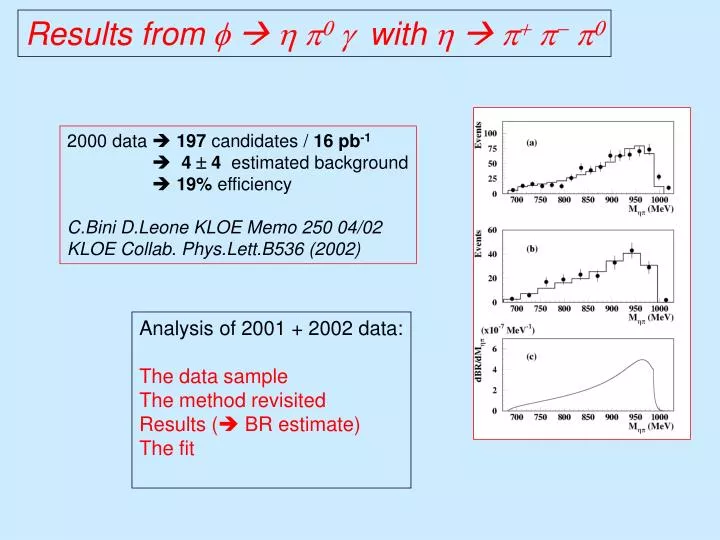
Results from f h p 0 g with h p + p - p 0. 2000 data 197 candidates / 16 pb -1 4 4 estimated background 19% efficiency C.Bini D.Leone KLOE Memo 250 04/02 KLOE Collab. Phys.Lett.B536 (2002). Analysis of 2001 + 2002 data:

E N D
Results fromf h p0 gwithh p+ p- p0 2000 data 197 candidates / 16 pb-1 4 4 estimated background 19% efficiency C.Bini D.Leone KLOE Memo 250 04/02 KLOE Collab. Phys.Lett.B536 (2002) Analysis of 2001 + 2002 data: The data sample The method revisited Results ( BR estimate) The fit
The Data Sample “good” runs: luminosity value ok good s value (a) used in kin.fits (b) for “phi-curve” removed trigger problems (KLOE Memo 281) “peak” runs 1018< s <1021 MeV 2001 2002 full sample140.4 264.9 “good” runs137.0 260.8 “peak” runs136.4 245.2 Full data sample 397.8 pb-1 “good” 381.6 pb-1 “peak” Lum (nb-1 / 0.2 MeV) vss
The Method (1 – kinematical fits) Selection procedure: Look for 2 tracks + 5 photons Kinematical fit 1 [ Etot = s , Ptot = PCM ] p(c21) > 5% Select combinations with p(c2comb) > 5% Kinematical fit 2 [ M(g1g2)=M(p0) , M(g3g4)=M(p0) , M(p+p-g1g2)=M(h) ] p(c22) > 5% and choose best combination E(g5) > 20 MeV MC Both kinematical fits are done numerically Using MINUIT (penalty function method) data The results has not to depend on the li 1/l (MeV)
The Method (2 - linearity) • After kinematical fit 1: • Look at M(gg) and M(p+p-gg) • distributions • [10 entries per event] • Mass peaks found p0 h w Data 2001 134.3 0.1 548.5 0.6 780.3 0.5 Data 2002 134.45 0.08 547.2 0.4 780.2 0.4 PDG values 134.9766 547.30 0.12 782.57 0.12 Old MC 134.6 0.3 548.3 0.5 New MC 132.9 0.3 544.8 0.5
The Method (3) p(c2) distributions: data – MC comparison New MC (15/05/03) good agreement using same resolution functions: s(E)/E = 5.7% / E s(t) = 55 ps / E 150 ps Old MC BUT serious linearity problems in new MC after second kin. fit [ M(hp0)meas – M(hp0)true ] (now should be ok) New MC
Results (1 – f line-shape + BR) Number of events 2001 2002 “good” sample 1424 2856 “peak” sample 1422 2759 • Comments: • 1 – we observe ~BW behaviour • hpg come from f 2 – discrepancy 2001 – 2002 [ ~ 2 s.d. ] but different s distribution 3 – estimate of BR (“peak” sample) s(f) = 3.34 mbarn BR(hp+p-p0) = 22.6 0.4 % PDG 2002 etot = 19.1% N(bckg) = (2 1)% BR(fhp0g) = (7.45 0.11 0.19)x10-5
Results (2 – spectra) • M(hp0) spectrum dynamics • of the decay a0 contribution. • 2001 vs 2002 • 2001+2002 vs. 2000 • [5 MeV vs 36 MeV binning] • Comparison of L-normalized • spectra.
Results (3 – angular distribution) • Expected angular distribution of the • radiated photon: • ( 1 + cos2qg) if hp is J=0 • Efficiency not flat in cosqg • (from MC) • Spectrum described by A(1 + cos2qg) + B Agreement data-MC (a0)
The fit Same combined fit done on 2000 data (Achasov function for a0 + rp) Free parameters: M(a0) g2(a0KK)/4p R=g(a0hp)/g(a0KK) BR(rp) Contributions to the c2 Data vs. fit “charged” spectrum “neutral” spectrum
The fit (results) Comments: c2 / dof still not good smearing of “charged” spectrum BR(rp) compatible with 0: “expected” is BR ~ 0.4 x 10⁻⁵ M(a0) ok a0 parameters in agreement with published fit
The Method (4 – efficiency) MC based efficiency + g eff. corrections + track eff. corrections (based on 2000 data and old MC) Overall efficiency vs. M(hp0) cosq(grad)
The Method (5 – background) The background is small ~ few %: 2t + 4/6 photons Results: (how many bckg events survive to the selection chain) 2 wp0 events 11 events on the “peak” sample 1 KSKL p0p0 p+p-p0 event 41 events on the “peak” sample No events from other channels < 100 events Check with distribution after fit-1: Describe M(p+p-gg) spectrum with Sum SIGNAL + BCKG
It works BUT: wp = wp x 4 Ksn = Ksn x 1.5 Estimated bckg Between 51 and 105 events / 4200 candidates: < 3% in the worst case This analysis needs “good” simulation of accidentals: Wait for new MC campaign