Climate-Air Quality Interactions: Impacts & Strategies
Discover the intricate relationship between climate and air quality, exploring key findings on aerosols, ozone, methane, and more. Learn about reducing emissions for a better environment and climate future.

Climate-Air Quality Interactions: Impacts & Strategies
E N D
Presentation Transcript
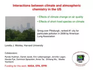
Interactions between Climate and Air Quality Hiram Levy II, Arlene M. Fiore, Larry W. Horowitz, Yuanyuan Fang, Yi Ming, Gabriel Vecchi Acknowledgments: Steve Howard and Jenise Swall, U.S. EPA 30th NATO/SPS International Technical Meeting on Air Pollution Modelling and its Application San Francisco, CA May 20, 2009
The U.S. smog problem is spatially widespread, affecting >150 million people [U.S. EPA, 2008] AEROSOLS (particulate matter) OZONE 4th highest daily max 8-hrin 2007 98th percentile 24-hr PM2.5 in 2007 Exceeds standard Exceeds standard http://www.epa.gov/air/airtrends/2008/report/TrendsReportfull.pdf
Radiative forcing of climate (1750 to present):Important contributions from air pollutants IPCC, 2007
Example # 1 - Double dividend of Methane Controls (Decreased greenhouse warming and improved air quality) AIR QUALITY: Number of U.S. summer grid-square days with O3 > 80 ppbv NOx OH CH4 50% anth. VOC 50% anth. NOx 1995 (base) 50% anth. CH4 Results are from GEOS-Chem global tropospheric chemistry model (4°x5°) CLIMATE: Radiative Forcing (W m-2) 50% anth. VOC 50% anth. CH4 50% anth. NOx Ozone precursors Fiore et al., GRL, 2002
Current Possible Methane Reductions 0.7 1.4 1.9 (industrialized nations) 10% of anth. emissions 20% of anth. emissions 0 20 40 60 80 100 120 Methane reduction (Mton CH4 yr-1) Take Home: 1. 0.7 ppb Ozone reduction at no cost 2. 1 ppb Ozone reduction via Methane control pays for itself (cost-savings + Carbon trading) 3. 1 ppb Ozone reduction over the eastern US via NOx control costs ~$1 billion yr-1 West & Fiore, ES&T, 2005
Methane Reduction Across A Range of Models Range across 18 models ~1.2 ppb decrease in N. Hemisphere surface O3 when CH4 decreased by 20% (1760 to 1408 ppb) N. Amer. Europe E. Asia S. Asia -20% Domestic Anthrop. Emissions -20% Foreign Anthrop. Emissions N. Amer. Europe E. Asia S. Asia N. Amer. Europe E. Asia S. Asia Key Results – Robust across models 1. Decreasing methane lowers global surface O3 background 2. Comparable local surface O3 decreases (ppb) from -20% intercontinental emissions of CH4 and NOx+NMVOC+CO; 3. “Traditional” local precursors more effective within source region Results from TF HTAP model intercomparison; Fiore et al., JGR, 2009
July surface O3 reduction from 30% decrease inanthropogenic CH4 emissions Globally uniform emission reduction Emission reduction in Asia 1. Ozone reduction is independent of location of methane reduction [pick the cheapest option] 2. Ozone reduction is generally largest in polluted regions [high nitrogen oxides] 3. Methane reduction is a win-win for climate and air quality Fiore et al., JGR, 2008
Pollution controls Example #2 - Direct Effect of Aerosols on Climate Scenarios for CO2 and short-lived greenhouse species Emissions of Short-lived Gases and Aerosols (A1B) CO2 concentrations 60 50 40 30 20 10 NOx (Tg N yr-1) A1B IPCC, 2001 250 200 150 100 50 SO2 (Tg SO2 yr-1) ppmv 25 20 15 10 5 0 BC (Tg C yr-1) Large uncertainty in future emission trajectories for short-lived species Horowitz, JGR, 2006 1880 1920 1960 2000 2040 2080
Up to 40% of U.S. warming in summer (2090s - 2000s) from changes in short-lived species From changing emissions of well-mixed greenhouse gases +short-lived species From changing emissions of short-lived species only Change in Summer Temperature 2090s-2000s (°C) Note: Warming from increases in BC + decreases in sulfate; depends critically on highly uncertain future emission trajectories Results from GFDL Climate Model [Levy et al., 2008]
Regional Radiative Forcing vs. Regional Temperature Response Radiative Forcing (2100 – 2001) Due To Short-lived Species Three Main Points: 1. Summertime central US appears to be very sensitive to climate change. 2. Radiative forcing and climate response are not spatially correlated 3. Asian emission controls may significantly impact US summertime warming Levy et al., JGR, 2008 global pattern-correlation coefficient of -0.172.
Example #3 - From Emissions to Clouds via Aerosol Indirect Effects Aerosol Direct Effects (TOA) ~0 W/m2 Key Issues - Post IPCC 2007 1. Now strong cooling from aerosol interactions with clouds (indirect effects). 2. Internal mixtures now reduce TOA direct aerosol effect to ~ 0. 3. Climate and Aerosols (emissions, chemical reactions, transport and removal) now all interact strongly through clouds. 4. Critical measurements are needed: optical properties of aerosols; magnitude of aerosol indirect effects. 5. Indirect effects may have significantly non-linear influences on temperature and precipitation. Aerosol Indirect effects (TOA) ~ -1.3 W/m2
SUMMARY OF Air Quality Climate 1. Methane reduction is a win-win for both air quality and climate. 2. Aerosol reduction is a double edged sword. 3. Indirect effects have introduced a major uncertainty in our quantitative understanding of the role played by aerosols. 4. Future emission projections are highly uncertain at best.
Strong relationship between weather and pollutionimplies that changes in climate will impact air quality
(1) Meteorology (stagnation vs. well-ventilated boundary layer) Degree of mixing strong mixing Boundary layer depth pollutant sources (2) Emissions (biogenic depend strongly on temperature; fires) VOCs T T Increase with T, drought? (3) Chemistry responds to changes in temperature, humidity NMVOCs CO, CH4 generally faster reaction rates O3 OH NOx + + How does climate affect air quality? PAN H2O
Pollution build-up during 2003 European heatwave GRG HEATWAVE Ozone CO Ventilation (low-pressure system) CO and O3 from airborne observations (MOZAIC) Above Frankfurt (850 hPa; ~160 vertical profiles Stagnant high pressure system over Europe (500 hPa geopotential anomaly relative to 1979-1995 for 2-14 August, NCEP) H Carlos Ordóñez, Toulouse, France Contribution to GEMS GEMS-GRG, subproject coordinated by Martin Schultz
Observations during 2003 European heatwave show enhanced biogenic VOC concentrations temperature (°C) = 95 °F = 86 °F concentration (pptv) BVOCs Measurements from August 2003 Tropospheric Organic Chemistry Experiment (TORCH) in Essex, UK, during hottest conditions ever observed in the UK to date c/o Dr. Alistair Lewis, University of York, UK Hogrefe et al., EM, 2005
Observed O3-temperature relationships:a useful test for building confidence in models? Example of information needed for statistical downscaling A. Fiore, private communication
Application of statistical downscaling to predict air quality response to future climate change Days in Summer (JJA) above 84ppb for Chicago area Solid lines – 10 year running ave. Dashed lines – single year GFDL (A1) HadCM3 (A2) PCM (A1) HadCM3 (B1) PCM (B1) GFDL(B1) 2000 2050 2100 Results based on historically observed meteorology-ozone relationships applied to climate model output for the Chicago area – Holloway et al., 2008
normalized to a +1°C 5 4 3 2 1 0 O3 response depends on local chemistry (available NOx) reaction humidity BVOC combined rates Impacts on surface O3 from T-driven increases in reaction rates, humidity, and BVOC emissions 3 p.m. O3 change (ppbv) in 3-day O3 episode with CMAQ model (4x4 km2), applying T change from 2xCO2 climate (changes in meteorology not considered) Surface ozone change ppbv ppbv Climate-driven O3 increases may counteract air quality improvements achieved via local anthropogenic emission reductions [Steiner et al., JGR, 2006]
Changes in land-use could have a large impact on future air quality (biogenic emissions) July isoprene emission capacity, normalized to 30°C (μg m-2 h-1) PRESENT DAY (1990-1999) FUTURE (2045-2054) • Conversion of forests to grasslands and crops decreases isoprene emissions (IPCC SRES A2 scenario) [Avise et al., ACP, 2009; Chen et al., ACP, 2009]
Models including impacts of changing climate on meteorology suggest increase in eastern U.S. pollution events due to fewer ventilating mid-latitude storms Tracer of anthropogenic pollution (July-August) Poleward shift in northern hemisphere summertime storm tracks for 2xCO2 2045-2052 A1B 1995-2002 m GFDL CM2.1 climate model e.g. in GISS global model (4°x5°) [Mickley et al., GRL, 2004] See also: Hogrefe et al., 2004, 2005; Jacob and Winner, 2009 and references therein
Isolate Climate Impact: Examine air quality in present vs. future climate in the newest GFDL atmospheric chemistry-climate model (AM3) Present Day Simulation (20 years) Climatological (1981-2000 mean) observed SSTs and sea ice (HadISST) Greenhouse gases at 1990 values Future Simulation (20 years) Present day 20 year mean SSTs, sea ice + IPCC AR-4 19-model mean changes for A1B scenario for 2081-2100 Greenhouse gases at 2090 values All simulations use annually-invariant emissions of ozone and aerosol precursors (except for lightning NOx), to isolate role of climate change
CHANGES IN SUMMER (JJA) PM2.5 AND 8-HOUR OZONE (FUTURE – BASE) PM2.5 24 hr. avg. OZONE daily max 8-hour avg.
AEROSOLS IN SURFACE AIR Future: 2081-2100 (climatological) Present: 1991-2000 (climatological) Individual symbols = individual years Line = 20-year average value 24-h monthly mean PM2.5 April through October
OZONE IN SURFACE AIR Future: 2081-2100 (climatological) Present: 1991-2000 (climatological) Individual symbols = individual years Line = 20-year average value Number of grid-square days with MDA8 ozone >75 ppb April through October
SUMMARY: Climate Air quality 1. Many possibilities for future air quality sensitivity to climate change (temperature, transport, BL mixing, biogenic sources, fires, ...) However 2. Quantitative understanding is highly uncertain. a. emission projections - (Who can predict 2050 conditions?) b. regional climate projections – (nothing in the last IPCC) c. aerosol-cloud indirect effects – (We have just started.) d. the next surprise – (There is always another one.) 3. My/our best current guess – Global warming won’t help.