Download
1 / 114
1.14k likes | 1.17k Vues
Explore the history of the Search for Extraterrestrial Intelligence (SETI) from its origins in 1959 to the future FOCAL space mission. Learn about mathematical models like the Statistical Drake Equation and Life as a b-Lognormal to understand civilizations in the Galaxy. Delve into the significance of Darwinian Evolution, Entropy, and exponential growth in shaping the evolution of life and civilizations. Discover how the Statistical Drake Equation is transformed to analyze an infinite number of factors and predict the distribution of communicating extraterrestrial civilizations. This comprehensive guide by Claudio Maccone, Director for Scientific Space Exploration, showcases the blend of mathematics and historical evolution driving the quest for contact with alien civilizations. ####

E N D
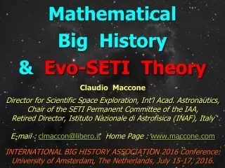
Mathematical Big History & Evo-SETI Theory Claudio Maccone Director for Scientific Space Exploration, Int’l Acad. Astronautics, Chair of the SETI Permanent Committee of the IAA, Retired Director, IstitutoNazionale di Astrofisica (INAF), Italy E-mail :clmaccon@libero.it Home Page : www.maccone.com INTERNATIONAL BIG HISTORY ASSOCIATION 2016 Conference: University of Amsterdam, The Netherlands, July 15-17, 2016.
History of SETI 1959:Giuseppe Cocconi & Philip Morrison’s seminal paper: «Searching for Interstellar Communications»,Nature184, 844-846 (19 September 1959) | doi:10.1038/184844a0 Cocconi Morrison
History of SETI 1960:First search at 1420 MHz (neutral hydrogen line) by Frank Drake, at the National Radio Astronomy Observatory in Green Bank, West Virginia (Project Ozma, 85 feet = 25.908 meter antenna). Frank Drake
History of SETI 2009:NASA’s “Kepler” space mission: >3000 planets.
Future of SETI: «FOCAL» mission “FOCAL” space mission beyond 550 AU ~ 3.17 light days ~ 14 times the Sun-Pluto distance: exploiting the Sun as a GRAVITATIONAL LENS to obtain MAGNIFIED RADIO PICTURES of an Alien Civilization and its planet.It would allow us to read the car plates on that planet!
TALK’s SCHEME 1/2 Part 1: STATISTICAL DRAKE QUATIONPart 2:STATISTICAL BIG HISTORY EQUATIONPart 3: LIFE as a b-LOGNORMAL (b=birth) Part 4: Darwinian EXPONENTIAL GROWTH Part 5: Geometric Brownian Motion (GBM) Part 6: Darwinian EVOLUTION as a GBMPart 7: ENTROPY as EVOLUTION MEASURE
TALK’s SCHEME 2/2 Part 8: Aztecs vs. Spaniards: ENTROPY in 1519Part 9: Future up to 10 million years Part 10: Mass ExtinctionsPart 11: ARBITRARY MEAN rather than GBMPart 12: Markov-Korotayev CUBIC process
Deterministic Drake Equation /1 • In 1961 Frank Drake introduced his famous “Drake equation” described at the web site http://en.wikipedia.org/wiki/Drake_equation. It yields the number N of communicating civilizations in the Galaxy: • Frank Donald Drake (b. 1930)
Deterministic Drake Equation /2 • The meaning of the seven factors in the Drake equation is well-known. • The middle factor fl is Darwinian Evolution. • In the classical Drake equation the seven factors are just POSITIVE NUMBERS. And the equation simply is the PRODUCT of these seven positive numbers. • It is claimed here that Drake’s approach is too “simple-minded”, since it does NOT yield the ERROR BAR associated to each factor!
STATISTICAL Drake Equation /1 • If we want to associate an ERROR BAR to each factor of the Drake equation then… • … we must regard each factor in the Drake equation as a RANDOM VARIABLE. • Then the number N of communicating civilizations also becomes a random variable. • This we call the STATISTICAL DRAKE EQUATION and studied in our mentioned reference paper of 2010 (Acta Astronautica, Vol. 67 (2010), pages 1366-1383)
STATISTICAL Drake Equation /2 • Denoting each random variable by capitals, the STATISTICAL DRAKE EQUATION reads • Where the D sub i (“D from Drake”) are the 7 random variables, and N is a random variable too (“to be determined”).
Extending the STATISTICAL Drake Equation to ANY NUMBER OF FACTORS /1 • Consider the statistical equation • This is the generalization of our Statistical Drake Equation to the product of ANY finite NUMBER of positive random variables. • Is it possible to determine the statistics of N ? • Rather surprisingly, the answer is “yes” !
Extending the STATISTICAL Drake Equation to ANY NUMBER OF FACTORS /2 • First, you obviously take the natural log of both sides to change the finite product into a finite sum • Second, to this finite sum one can apply the CENTRAL LIMIT THEOREM OF STATISTICS. It states that, in the limit for an infinite sum, the distribution of the left-hand-side is NORMAL. • This is true WHATEVER the distributions of the random variables in the sum MAY BE.
SOLVING the STATISTICAL Drake Equation for INFINITELY MANY FACTORS • So, the random variable on the left is NORMAL, i.e. • Thus, the random variable N under the log must be LOG-NORMAL and its distribution is determined! • One must, however, determine the mean value and variance of this log-normal distribution in terms of the mean values and variances of the factor random variables. This is DIFFICULT. But it can be done, for example, by a suitable numeric code that this author wrote in MathCad language.
Conclusion about the Drake equation:The number of Signaling Civilizations is LOGNORMALLY distributed • Our Statistical Drake Equation, now Generalized to any number of factors, embodies as a special case the Statistical Drake Equation with just 7 factors. • The conclusion is that the random variable N (the number of communicating ET Civilizations in the Galaxy) is LOG-NORMALLY distributed. • The classical “old pure-number Drake value” of N is now replaced by the MEAN VALUE of such a log-normal distribution. • But we now also have an ERROR BAR around it !
REFERENCE PAPER : • The Statistical Drake Equation • Acta Astronautica, V. 67 (2010), p. 1366-1383.
REFERENCE PAPER : • SETI as a Part of Big History • Acta Astronautica, Vol.101 (2014), pag. 67-80.
THE BIG HISTORY EQUATION is 1) The DRAKE equation (yielding the Evolution of Life on Earth since -3.5 billion years ago) 2) PLUS the BEGINNING TERM i.e. the cosmological evolution of the Universe PRIOR to -3.5 billion years. • In fact, the WHOLE UNIVERSE (and NOT just the Milky Way) evolved since the Big Bang
BIG HISTORY EQUATION • Where is the (unknown) number of Galaxies supposed to exist in the entire Universe. • The probability distribution of the new random variable “Number of Civilizations in the Universe” is a lognormal, but we don’t know when it started... • …at least until we will know a sufficient number of Alien Civilizations!
BIG HISTORY: an exponential in the growing number of Civilizations?We won’t know until... The SETI scientists will succeedin finding the first few Alien Civilizations
BIG HISTORY: an exponential in the growing number of Civilizations?
BIG HISTORY: an exponential in the growing number of Civilizations?
Part 3:b-LOGNORMALSas the LIFE-TIME of a cell, of an animal, of a human, a civilization (f sub i) even ET (f sub L)
LIFE as a FINITE b-LOGNORMAL • The lifetime of a cell, an animal, a human, a civilization can be modeled as a b-lognormal with tail REPLACED at senility by the descending TANGENT. The interception at time axis is DEATH=d.
LIFE as a FINITE b-LOGNORMAL • The equation of a INFINITE b-lognormal is : • The lifetime of a cell, an animal, a human, a civilization can be modeled as a FINITE b-lognormal: namely an infinite b-lognormal whose TAIL has been REPLACED at senility by the descending TANGENT STRAIGHT LINE. The interception of this straight line at time axis is DEATH=d.
Let a = increasing inflexion, s = decreasing inflexion. • Then any b-lognormal has birth time (b), adolescencetime (a), peak time (p) and senility time (s). • Rome’s civilization: b=-753, a=-146, p=59, s=235. • HISTORY FORMULAE : GIVEN (b, s, d) it is always possible to compute the corresponding b-lognormal by virtue of the following two HISTORY FORMULAE : HISTORY FORMULAE
Let a = increasing inflexion, s = decreasing inflexion. • Then any b-lognormal has birth time (b), adolescencetime (a), peak time (p) and senility time (s). • Rome’s civilization: b=-753, a=-146, p=59, s=235. LIFE as INFINITE b-LOGNORMAL
LIFE as a FINITE b-LOGNORMAL • ANY FINITE LIFE may be modeled as a b-lognormal with tail REPLACED at senility by the descending TANGENT. The interception at time axis is DEATH=d. • (e.g. for Rome civilization one has b=-753, d=476)
Given TWO POINTS with coordinates : • The EXPONENTIAL must have: Two EXPONENTIAL ENVELOPES
Part 4:PEAK-LOCUS THEOREM:Darwinian EXPONENTIAL GROWTH as LOCUS of b-LOGNORMAL PEAKS
REFERENCE PAPER : • A Mathematical Model for Evolution and SETI • Origins of Life and Evolution of Biospheres (OLEB), Vol. 41 (2011), pages 609-619.
Darwinian EXPONENTIAL GROWTH • Life on Earth evolved since 3.5 billion years ago. • The number of Species GROWS EXPONENTIALLY: assume that today 50 million species live on Earth • Then:
Darwinian EXPONENTIAL GROWTH • Life on Earth evolved since 3.5 billion years ago. • The number of Species GROWS EXPONENTIALLY: assume that today 50 million species live on Earth • Then: • with:
EXPONENTIAL as “ENVELOPE” of b-LOGNORMALS • Each b-lognormal has its peak on the exponential. • PRACTICALLY an “Envelope”, though not so formally.
b-LOGNORMALS i.e. LOGNORMALS starting at b=birth • b-lognormals are just lognormals starting at any finite positive instant b>0, that is supposed to be known. • b-lognormals are thus a family of probability density functions with three real and positive parameters: m, s, and b.