Mastering Ray-Tracing: An In-Depth Overview
Dive deep into the world of ray-tracing through recursive ray tracing, shadow feelers, and Snell's Law for refraction. Learn when to stop for optimal results and the essentials of light transport, local illumination, and shadow feelers. Discover the complexities of reflection, computation of reflectance, and perfect specular transmission. Explore the inclusion of transparent objects in ray tracing, the challenges faced, and methods to optimize performance. Enhance your understanding of specular reflections and the limitations of ray tracing simulations.

Mastering Ray-Tracing: An In-Depth Overview
E N D
Presentation Transcript
Overview • Recursive Ray Tracing • Shadow Feelers • Snell’s Law for Refraction • When to stop!
( ) m ( å ( ) ) M = + I k I k n l k h n + × × , r a i j d j s j = 1 j Recap: Local Illumination • Ambient, diffuse & specular components • The sum is over the specular and diffuse components for each light I a
Correcting for Non-Visible Lights N H E L surface
Where Sj is the result of intersecting the ray L with the scene objects • Note consider your intersection points along the ray L carefully • Hint – they might be beyond the light!
Recursive Ray-Tracing • We can simulate specular-specular transmission elegantly by recursing and casting secondary rays from the intersection points • We must obviously chose a termination depth to cope with multiple reflections
Introducing Reflection N H R • Where E L surface
Computing the reflection direction N E • Ideal reflection • = • R same plane as V and N R = aE + bN • E.N = N.R = a(N.E)+b • If a = -1, b = 2N.E R = -E + 2(N.E)N R
Computing Reflectance • Where Ilocal is computed as before • Ray r' is formed from intersection point and the direction R and is cast into the scene as before
p’’ L2 R2 R1 p p’ L1 Recursive Ray Tracing
Pseudo Code Color RayTrace(Point p, Vector direction, int depth) { Point pd /* Intersection point */ Boolean intersection if (depth > MAX) return Black intersect(p,direction, &pd, &intersection) if (!intersection) return Background Ilocal = kaIa + Ip.v.(kd(n.l) + ks.(h.n)m) return Ilocal + kr*RayTrace(pd, R, depth+1) } Normally kr = ks
Perfect Specular Transmission N H E R Snell’s Law L 1 is index of refraction 2 T ß
Using Snell’s Law • Using this law it is possible to show that: • Note that if the root is negative then total internal reflection has occurred and you just reflect the vector as normal
T2 p’’ L2 R2 R1 p p’ T1 L1 Recursive Ray Tracing Including Transparent Objects
New Pseudo Code Color RayTrace(Point p, Vector D, int depth) { Point pd /* Intersection point */ Boolean intersection if (depth > MAX) return Black intersect(p,direction, &pd, &intersection) if (!intersection) return Background Ilocal = kaIa + Ip.v.(kd(n.l) + ks.(h.n)m) return Ilocal + kr*RayTrace(pd, R, depth+1) + kt*RayTrace(pd, T, depth+1) }
Direct Specular Transmission N • A transparent surface can be illuminated from behind and this should be calculated in Ilocal H' E L
Calculating H' • Use H‘ instead of H in specular term
Remark • Specular and transmission only • What should be added to consider diffuse reflection? • Why it’s expensive • Intersection of rays with polygons (90%) • How to reduce the cost? • Reduce the number of rays • Reduce the cost on each ray • First check with bounding box of the object • Methods to sort the scene and make it faster
Summary • Recursive ray tracing is a good simulation of specular reflections • We’ve seen how the ray-casting can be extended to include shadows, reflections and transparent surfaces • However this is a very slow process and still misses some types of effect!