Computing Engine Choices

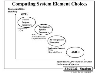
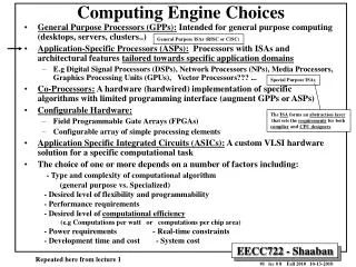
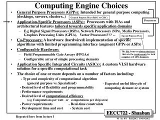
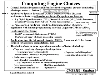
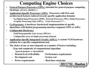
1. Computing Engine Choices • General Purpose Processors (GPPs): Intended for general purpose computing (desktops, servers, clusters..) • Application-Specific Processors (ASPs): Processors with ISAs and architectural features tailored towards specific application domains • E.g Digital Signal Processors (DSPs), Network Processors (NPs), Media Processors, Graphics Processing Units (GPUs), Vector Processors??? ... • Co-Processors: A hardware (hardwired) implementation of specific algorithms with limited programming interface (augment GPPs or ASPs) • Configurable Hardware: • Field Programmable Gate Arrays (FPGAs) • Configurable array of simple processing elements • Application Specific Integrated Circuits (ASICs): A custom VLSI hardware solution for a specific computational task • The choice of one or more depends on a number of factors including: - Type and complexity of computational algorithm (general purpose vs. Specialized) - Desired level of flexibility - Performance requirements - Development cost - System cost - Power requirements - Real-time constrains

2. Computing Engine Choices • E.g Digital Signal Processors (DSPs), • Network Processors (NPs), • Media Processors, • Graphics Processing Units (GPUs) General Purpose Processors (GPPs): Flexibility Application-Specific Processors (ASPs) Configurable Hardware Selection Factors: Co-Processors - Type and complexity of computational algorithms (general purpose vs. Specialized) - Desired level of flexibility - Performance - Development cost - System cost - Power requirements - Real-time constrains Application Specific Integrated Circuits (ASICs) Performance

3. Digital Signal Processor (DSP) Architecture • Classification of Processor Applications • Requirements of Embedded Processors • DSP vs. General Purpose CPUs • DSP Cores vs. Chips • Classification of DSP Applications • DSP Algorithm Format • DSP Benchmarks • Basic Architectural Features of DSPs • DSP Software Development Considerations • Classification of Current DSP Architectures and example DSPs: • Conventional DSPs: TI TMSC54xx • Enhanced Conventional DSPs: TI TMSC55xx • VLIW DSPs: TI TMS320C62xx, TMS320C64xx • Superscalar DSPs: LSI Logic ZSP400 DSP core

4. Processor Applications • General Purpose Processors (GPPs) - high performance. • RISC or CISC: Intel P4, IBM Power4, SPARC, PowerPC, MIPS ... • Used for general purpose software • Heavy weight OS - Windows, UNIX • Workstations, Desktops (PC’s), Clusters • Embedded processors and processor cores • e.g: Intel XScale, ARM, 486SX, Hitachi SH7000, NEC V800... • Often require Digital signal processing (DSP) support or other application-specific support (e.g network, media processing) • Single program • Lightweight, often realtime OS or no OS • Examples: Cellular phones, consumer electronics .. (e.g. CD players) • Microcontrollers • Extremely cost/power sensitive • Single program • Small word size - 8 bit common • Highest volume processors by far • Examples: Control systems, Automobiles, toasters, thermostats, ... Increasing Cost/Complexity Increasing volume Examples of Application-Specific Processors

5. Processor Markets $30B 32-bit micro $5.2B/17% $1.2B/4% 32 bit DSP $10B/33% DSP 16-bit micro $5.7B/19% $9.3B/31% 8-bit micro

6. The Processor Design Space Application specific architectures for performance Embedded processors Microprocessors GPPs Real-time constraints Specialized applications Low power/cost constraints Performance is everything & Software rules Performance Microcontrollers Cost is everything Processor Cost

7. Requirements of Embedded Processors • Usually must meet real-time constraints • Optimized for a single program - code often in on-chip ROM or off chip EPROM • Minimum code size (one of the motivations initially for Java) • Performance obtained by optimizing datapath • Low cost • Lowest possible area • High computational efficiency: Computation per unit area • Implementation technology usually behind the leading edge • High level of integration of peripherals (System-on-Chip -SoC- approach reduces system cost) • Fast time to market • Compatible architectures (e.g. ARM family) allows reusable code • Customizable cores (System-on-Chip, SoC). • Low power if application requires portability

8. Embedded Processors Area of processor cores = Cost Nintendo processor Cellular phones

9. Embedded Processors Another figure of merit: Computation per unit area Nintendo processor Cellular phones

10. Embedded Processors Code size • If a majority of the chip is the program stored in ROM, then code size is a critical issue • Variable length instruction encoding common: • e.g. the Piranha has 3 sized instructions - basic 2 byte, and 2 byte plus 16 or 32 bit immediate

11. Embedded System Runs a few applications often known at design time Not end-user programmable Operates in fixed run-time constraints that must be met, additional performance may not be useful/valuable (e.g. real-time sampling rate) Differentiating features: Application-specific capability (e.g DSP) power cost speed (must be predictable) Embedded Systems vs. General Purpose Computing General Purpose Computing • Intended to run a fully general set of applications • End-user programmable • Faster is always better • Differentiating features • speed (need not be fully predictable) • Superscalar: dynamic scheduling, speculation, branch prediction, cache. • cost (largest component power)

12. Evolution of GPPs and DSPs • General Purpose Processors (GPPs) trace roots back to Eckert, Mauchly, Von Neumann (ENIAC) • DSP processors are microprocessors designed for efficient mathematical manipulation of digital signals. • DSP evolved from Analog Signal Processors (ASPs), using analog hardware to transform physical signals (classical electrical engineering) • ASP to DSP because • DSP insensitive to environment (e.g., same response in snow or desert if it works at all) • DSP performance identical even with variations in components; 2 analog systems behavior varies even if built with same components with 1% variation • Different history and different applications requirements led to different terms, different metrics, architectures, some new inventions.

13. DSP vs. General Purpose CPUs • DSPs tend to run one program, not many programs. • Hence OSes (if any) are much simpler, there is no virtual memory or protection, ... • DSPs usually run applications with hard real-time constraints: • DSP must meet application signal sampling rate computational requirements: • A faster DSP is overkill (higher DSP cost, power..) • You must account for anything that could happen in a time slot (DSP algorithm inner-loop, data sampling rate) • All possible interrupts or exceptions must be accounted for and their collective time be subtracted from the time interval. • Therefore, exceptions are BAD. • DSPs usually process infinite continuous data streams: • Requires high memory bandwidth for streaming real-time data samples • The design of DSP architectures and ISAs driven by the requirements of DSP algorithms. • Thus DSPs are application-specific processors

14. DSP vs. GPP • The “MIPS/MFLOPS” of DSPs is speed of Multiply-Accumulate (MAC). • MAC is common in DSP algorithms that involve computing a vector dot product, such as digital filters, correlation, and Fourier transforms. • DSP are judged by whether they can keep the multipliers busy 100% of the time and by how many MACs are performed in each cycle. • The "SPEC" of DSPs is 4 algorithms: • Inifinite Impule Response (IIR) filters • Finite Impule Response (FIR) filters • FFT, and • convolvers • In DSPs, target algorithms are important: • Binary compatibility not a major issue • High-level Software is not as important in DSPs as in GPPs. • People still write in assembly language for a product to minimize the die area for ROM in the DSP chip.

15. Types of DSP Processors • 32-BIT FLOATING POINT (5% of market): • TI TMS320C3X, TMS320C67xx • AT&T DSP32C • ANALOG DEVICES ADSP21xxx • Hitachi SH-4 • 16-BIT FIXED POINT (95% of market): • TI TMS320C2X, TMS320C62xx • Infineon TC1xxx (TriCore1) • MOTOROLA DSP568xx, MSC810x • ANALOG DEVICES ADSP21xx • Agere Systems DSP16xxx, Starpro2000 • LSI Logic LSI140x (ZPS400) • Hitachi SH3-DSP • StarCore SC110, SC140

16. DSP Cores vs. Chips DSP are usually available as synthesizable cores or off-the- shelf packaged chips • Synthesizable Cores: • Map into chosen fabrication process • Speed, power, and size vary • Choice of peripherals, etc. (SoC) • Requires extensive hardware development effort. • Off-the-shelf packaged chips: • Highly optimized for speed, energy efficiency, and/or cost. • Limited performance, integration options. • Tools, 3rd-party support often more mature

17. Time Frame Approach Primary Application Enabling Technologies Early 1970’s · · · Discrete logic Non-real time Bipolar SSI, MSI procesing · FFT algorithm · Simulation Late 1970’s · · · Building block Military radars Single chip bipolar multiplier · · Digital Comm. Flash A/D m m Early 1980’s · · · Single Chip DSP P Telecom P architectures · Control · NMOS/CMOS Late 1980’s · · · Function/Application Computers Vector processing specific chips · · Communication Parallel processing Early 1990’s · · · Multiprocessing Video/Image Processing Advanced multiprocessing · VLIW, MIMD, etc. Late 1990’s · · · Single-chip Wireless telephony Low power single-chip DSP multiprocessing · Internet related · VLIW/Multiprocessing DSP ARCHITECTUREEnabling Technologies

18. Texas Instruments TMS320 Family Multiple DSP P Generations

19. Digital audio applications MPEG Audio Portable audio Digital cameras Cellular telephones Wearable medical appliances Storage products: disk drive servo control Military applications: radar sonar DSP Applications • Industrial control • Seismic exploration • Networking: (Telecom infrastructure) • Wireless • Base station • Cable modems • ADSL • VDSL • …... Current DSP Killer Applications: Cell phones and telecom infrastructure

20. DSP Applications

21. Another Look at DSP Applications • High-end • Military applications (e.g. radar/sonar) • Wireless Base Station - TMS320C6000 • Cable modem • gateways • Mid-end • Industrial control • Cellular phone - TMS320C540 • Fax/ voice server • Low end • Storage products - TMS320C27 (hard drive controllers) • Digital camera - TMS320C5000 • Portable phones • Wireless headsets • Consumer audio • Automobiles, toasters, thermostats, ... Increasing Cost Increasing volume

22. DSP range of applications

23. CELLULAR TELEPHONE SYSTEM 1 2 3 4 5 6 7 8 9 0 415-555-1212 CONTROLLER RF MODEM PHYSICAL LAYER PROCESSING BASEBAND CONVERTER A/D SPEECH ENCODE SPEECH DECODE DAC

24. HW/SW/IC PARTITIONING MICROCONTROLLER 1 2 3 4 5 6 7 8 9 0 415-555-1212 CONTROLLER RF MODEM PHYSICAL LAYER PROCESSING BASEBAND CONVERTER ASIC A/D SPEECH ENCODE SPEECH DECODE DAC DSP ANALOG IC

25. S/P RAM DMA DSP CORE Mapping Onto System-on-Chip (SoC) S/P phone book keypad intfc protocol DMA control RAM µC speech quality enhancment voice recognition ASIC LOGIC RPE-LTP speech decoder de-intl & decoder Viterbi equalizer demodulator and synchronizer

26. Example Wireless Phone Organization C540 (DSP) ARM7 (µC)

27. Radio Modem Multimedia I/O Architecture Embedded Processor Sched ECC Pact Interface Low Power Bus FB Video Decomp Fifo Fifo Pen SRAM Data Flow Graphics Audio Video

28. Graphics Out Uplink Radio Video I/O Downlink Radio Voice I/O Pen In µP Video Unit custom Coms Memory DSP Multimedia System-on-Chip (SoC) e.g. Multimedia terminal electronics • Future chips will be a mix of processors, memory and dedicated hardware for specific algorithms and I/O (ASIC)

29. DSP Algorithm Format • DSP culture has a graphical format to represent formulas. • Like a flowchart for formulas, inner loops, not programs. • Some seem natural:  is add, X is multiply • Others are obtuse: z–1 means take variable from earlier iteration (delay). • These graphs are trivial to decode

30. DSP Algorithm Notation • Uses “flowchart” notation instead of equations • Multiply is or X • Add is or + • Delay/Storage is or or Delay z–1 D

31. Typical DSP Algorithm:Finite-Impulse Response (FIR) Filter • Filters reduce signal noise and enhance image or signal quality by removing unwanted frequencies. • Finite Impulse Response (FIR) filters compute: where • x is the input sequence • y is the output sequence • h is the impulse response (filter coefficients) • N is the number of taps (coefficients) in the filter • Output sequence depends only on input sequence and impulse response.

32. Typical DSP Algorithms:Finite-impulse Response (FIR) Filter • N most recent samples in the delay line (Xi) • New sample moves data down delay line • Filter “Tap” is a multiply-add • Each tap (N taps total) nominally requires: • Two data fetches • Multiply • Accumulate • Memory write-back to update delay line • Special addressing modes (e.g modulo) • Goal: At least 1 FIR Tap / DSP instruction cycle • Requires real-time data sample streaming • Predictable data bandwidth/latency • Special addressing modes • Repetitive computations, multiply and accumulate (MAC) • Requires efficient MAC support

33. X . . . . hN-1 hN-2 h1 h0 Y FINITE-IMPULSE RESPONSE (FIR) FILTER A Tap Goal: at least 1 FIR Tap / DSP instruction cycle DSP must meet application signal sampling rate computational requirements: A faster DSP is overkill

34. Sample Computational Rates for FIR Filtering (4.37 GOPs) (23.3 GOPs) 1-D FIR has nop = 2N and a 2-D FIR has nop = 2N2. OP = Operation • DSP must meet application signal sampling rate computational requirements: • A faster DSP is overkill (higher DSP cost, power..)

35. FIR filter on (simple) General Purpose Processor loop: lw x0, 0(r0) lw y0, 0(r1) mul a, x0,y0add y0,a,b sw y0,(r2) inc r0 inc r1 inc r2 dec ctr tst ctr jnz loop • Problems: • Bus / memory bandwidth bottleneck, • control/loop code overhead • No suitable addressing modes, instructions - • e.g. multiply and accumulate (MAC) instruction

36. Typical DSP Algorithms:Infinite-Impulse Response (IIR) Filter • Infinite Impulse Response (IIR) filters compute: • Output sequence depends on input sequence, previous outputs, and impulse response. • Both FIR and IIR filters • Require vector dot product (multiply-accumulate) operations • Use fixed coefficients • Adaptive filters update their coefficients to minimize the distance between the filter output and the desired signal.

37. Typical DSP Algorithms:Discrete Fourier Transform • The Discrete Fourier Transform (DFT) allows for spectral analysis in the frequency domain. • It is computed as for k = 0, 1, … , N-1, where • x is the input sequence in the time domain • y is an output sequence in the frequency domain • The Inverse Discrete Fourier Transform is computed as • The Fast Fourier Transform (FFT) provides an efficient method for computing the DFT.

38. Typical DSP Algorithms:Discrete Cosine Transform (DCT) • The Discrete Cosine Transform (DCT) is frequently used in image & video compression (e.g. JPEG, MPEG-2). • The DCT and Inverse DCT (IDCT) are computed as: where e(k) = 1/sqrt(2) if k = 0; otherwise e(k) = 1. • A N-Point, 1D-DCT requires N2MAC operations.

39. DSP BENCHMARKS • DSPstone: University of Aachen, application benchmarks • ADPCM TRANSCODER - CCITT G.721, REAL_UPDATE, COMPLEX_UPDATES • DOT_PRODUCT, MATRIX_1X3, CONVOLUTION • FIR, FIR2DIM, HR_ONE_BIQUAD • LMS, FFT_INPUT_SCALED • BDTImark2000: Berkeley Design Technology Inc • 12 DSP kernels in hand-optimized assembly language: • FIR, IIR, Vector dot product, Vector add, Vector maximum, FFT …. • Returns single number (higher means faster) per processor • Use only on-chip memory (memory bandwidth is the major bottleneck in performance of embedded applications). • EEMBC (pronounced “embassy”): EDN Embedded Microprocessor Benchmark Consortium • 30 companies formed by Electronic Data News (EDN) • Benchmark evaluates compiled C code on a variety of embedded processors (microcontrollers, DSPs, etc.) • Application domains: automotive-industrial, consumer, office automation, networking and telecommunications

40. 4th Generation 3rd Generation 2nd Generation 1st Generation

41. Basic Architectural Features of DSPs • Data path configured for DSP algorithms • Fixed-point arithmetic (most DSPs) • Modulo arithmetic (saturation to handle overflow) • MAC- Multiply-accumulate unit(s) • Hardware rounding support • Multiple memory banks and buses - • Harvard Architecture • Multiple data memories • Specialized addressing modes • Bit-reversed addressing • Circular buffers • Specialized instruction set and execution control • Zero-overhead loops • Support for fast MAC • Fast Interrupt Handling • Specialized peripherals for DSP Usually with no data cache for predictable fast data sample streaming To meet real-time signal sampling/processing constraints

42. DSP Data Path: Arithmetic • DSPs dealing with numbers representing real world signals=> Want “reals”/ fractions • DSPs dealing with numbers for addresses=> Want integers • Support “fixed point” as well as integers . -1 Š x < 1 S radix point . –2N–1 Š x < 2N–1 S radix point Usually 16-bit

43. DSP Data Path: Precision • Word size affects precision of fixed point numbers • DSPs have 16-bit, 20-bit, or 24-bit data words • Floating Point DSPs cost 2X - 4X vs. fixed point, slower than fixed point • DSP programmers will scale values inside code • SW Libraries • Separate explicit exponent • “Blocked Floating Point” single exponent for a group of fractions • Floating point support simplify development for high-end DSP applications.

44. DSP Data Path: Overflow • DSP are descended from analog : • Modulo Arithmetic. • Set to most positive (2N–1–1) or most negative value(–2N–1) : “saturation” • Many DSP algorithms were developed in this model. 2N–1–1 Due to physical nature of signals –2N–1

45. DSP Data Path: Multiplier • Specialized hardware performs all key arithmetic operations in 1 cycle, including: • Shifters • Saturation • Guard bits • Rounding modes • Multiplication/addition • 50% of instructions can involve multiplier=> single cycle latency multiplier • Need to perform multiply-accumulate (MAC) fast • n-bit multiplier => 2n-bit product

46. Multiplier Multiplier Shift ALU ALU Accumulator Accumulator G DSP Data Path: Accumulator • Don’t want overflow or have to scale accumulator • Option 1: accumalator wider than product: “guard bits” • Motorola DSP: 24b x 24b => 48b product, 56b Accumulator • Option 2: shift right and round product before adder

47. DSP Data Path: Rounding • Even with guard bits, will need to round when storing accumulator into memory • 3 DSP standard options (supported in hardware) • Truncation: chop results=> biases results up • Round to nearest: < 1/2 round down,  1/2 round up (more positive)=> smaller bias • Convergent: < 1/2 round down, > 1/2 round up (more positive), = 1/2 round to make lsb a zero (+1 if 1, +0 if 0)=> no biasIEEE 754 calls this round to nearest even

48. DSP Processor Specialized hardware performs all key arithmetic operations in 1 cycle. e.g MAC Hardware support for managing numeric fidelity: Shifters Guard bits Saturation Data Path Comparison General-Purpose Processor • Multiplies often take>1 cycle • Shifts often take >1 cycle • Other operations (e.g., saturation, rounding) typically take multiple cycles.

49. TI 320C54x DSP (1995) Functional Block Diagram Multiple memory banks and buses MAC Unit Hardware support for rounding/saturation

50. Instruction Memory Data Memory First Commercial DSP (1982): Texas Instruments TMS32010 • 16-bit fixed-point arithmetic • Introduced at 5Mhz (200ns) instruction cycle. • “Harvard architecture” • separate instruction, data memories • Accumulator • Specialized instruction set • Load and Accumulate • Two-cycle (400 ns) Multiply-Accumulate (MAC) time. Processor Datapath: Mem T-Register Multiplier P-Register ALU Accumulator