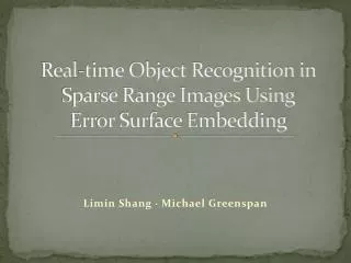
Real-time Object Recognition in Sparse Range Images Using Error Surface Embedding
Real-time Object Recognition in Sparse Range Images Using Error Surface Embedding. Limin Shang · Michael Greenspan. Outline. Introduction 3D registration ICP algorithm Creating error surfaces Curvilinear component analysis Reducing storage Embedding Pose determination

Real-time Object Recognition in Sparse Range Images Using Error Surface Embedding
E N D
Presentation Transcript
Real-time Object Recognition in Sparse Range Images UsingError Surface Embedding Limin Shang · Michael Greenspan
Outline • Introduction • 3D registration • ICP algorithm • Creating error surfaces • Curvilinear component analysis • Reducing storage • Embedding • Pose determination • Multiple object detection • Acceleration • Experiments • Conclusion
Introduction • Many approach to 2-d image recognition had some success but sensitive to shadow and illumination • Using range sensors does not suffer from above problems • Model-based 3-d object recognition techniques are robust to clutter and occlusions • Most algorithms are sensitive to noise
3D Registration • Produce point clouds combination from two or more point clouds
ICP Algorithm • ICP algorithm is used to find minimum of specified error function in this paper: R: rotation matrix T: translation vector Error :
ICP Algorithm • Iterative Closest Point • Give two clouds of points • Associate points by the nearest neighbor criteria. • Estimate transformation parameters using a mean square cost function. • Transform the points using the estimated parameters. • Iterative steps
ICP Algorithm • Depending on initial estimation, ICP will converge to either global minimum or one of local minima • In this paper, ICP is used to find local min, which are used to construct “compact feature vectors”, the performance is not related whether it is converge to global min or not • Compare the “compact feature vectors” between database data and runtime data later
Number of views • Get range image from different sides of object • Set three rotational increments to (20,20,30) degree • 1st dim : normal to 2nd dim • 2nd dim : camera self rotation • 3rd dim : rotate camera around the line of sight • Total number of views is 18x10x12 = 2160
Error Surface • P: range image of a model • Θ : 6-dim comprising 3-d rotation and 3-d translation parameter • Convolve P over complete pose space -> 7D hyper surface (time-consuming, hard to visualize) • Convolve P over 3-d translation parameter -> 4-d hyper surface (good enough)
Curvilinear Component Analysis • Used to reduce 4-d error space to 3-d surface for visualization, minimizing error function • PCA : works when dependencies between dimensions are strictly linear • CCA : F is weighting function (depending on di,jp )
Testing of robustness • Zero-mean Gaussian noise (σ = 15mm, size of original object is 200mm) • Sparse range data (75 points picked from 1000) • Data with simulated outlier (1000 additional points)
Robustness ↑ Surface error when using original data Surface error for tests→
Robustness • The error surfaces are similar regardless to degradation of input range image • Correlation between error surfaces X and Y can be calculated as • Figures show robustness of this method
Reducing search time • It would be expensive to save 2160 views per model • For each Views (Pi), the closest local minimum for Θic is calculated by executing ICP from its centroid, then take translation part tic from Θic , and used as the origin of the local coordinate system • Each Pi then perturbed to a set of K initial poses Θi0 around the calculated origin • In this dataset, K = 30 is tested to be effective
Perturbation • The perturbation is chosen to be distributed uniformly in the translational subspace • Let rm represents max radius of 3d model • Magnitude range of perturbation is (-rm, rm), with increment rm/2 • Results in 53 = 125 perturbation vectors • After applying the perturbations, ICP is allowed to execute in small number of iterations (more chances to converge)
Embedding • Run ICP with K initial poses produces K final poses • Combine K of Θs in final poses to be Ei • Such Ei is called an embedding of error surface Si, and used to compactly and descriptively represent a unique view Pi
Pose Determination • Above process is repeated at runtime for image data P: • Get Θ by local minima with ICP • Translate image P by translational term tpc so local minimum lies at the origin • Transfer to each of K perturbations • Get embeddings Ep and compare with Ei (preprocessed database)
Pose Determination • The similarity of two embeddings is calculated as:
Pose Determination • The closest view matching current image is identified by sum of similarity
Multiple Object Detection • In previous steps, it is assumed that there is only one object under consideration • Straightforward application: • Build database using multiple objects • Calculate expensively at runtime • Author purposed a solution : • Use generic model • In preprocessing, instead of convolving views with a model of itself, convolve views with single generic model • At runtime, only a single embedding of error surface of image is required to be calculated and compare against database
Generic Model Example of a generic model
Generic Model • Generate 120 spheres randomly in the bounding box DbxDbxDb • Radii of spheres are randomly in range of Db/10 to Db/4 • As long as complexity of generic model exceeds a certain degree (number of spheres is large enough), the differences among results using different generic model is minor
Acceleration • Divide translational subspace using quantize vector(Dd/15, Dd/15, Dd/15) • Total K hash tables are built for each of K local minima in a preprocessing step • Compare only in the same hash bucket • Vote with all members in the same bucket • Set vote threshold to be 0.5 x K, if embedding receive vote exceeding this, then use for distance calculation
Experements • Max iteration of ICP is set to 3 • Running on multicore computer • Uses the shown generic model (4000 points)
Experiments • Used range images (Mian et al. 2006) • 21 range images of chef, 15 images for chicken • 20 images for T-rex, 15 images for parasaurlophus ↑cylinder-like shape
Experiments • Another 5 objects: • Angel, Big bird, Gnome, Watermelon Kid, Zoe
Experiments 60 simulated data objects
Experiments Misrecognition between jeep and tank
Experiments Robustness vs sparseness/noise/outliers
Experiments • Different generic model • Number of spheres = 30,60,90,120,150 • Each contain 4000 points
Experiments • Used Princeton Shape Benchmark • 907 models divided into 90 classes (training) • Other 907 models divided into 92 classes (testing) • Testing on different K value
Experiments • Recognition peak at K=60 • Slightly decreased from 70 to 120 • Reduces pose determination rate for symmetric objects(sword ,tools, hourglass)
Conclusion • The purposed method is efficient and robust to data sparseness, outliers, and measurements error • Runs ICP in 3 iterations • Runs at 122 FPS • 98% recognition and 97% pose estimation rate in 60 objects