Object Recognition using Local Descriptors
Object Recognition using Local Descriptors. Javier Ruiz-del-Solar, and Patricio Loncomilla Center for Web Research Universidad de Chile. Outline. Motivation & Recognition Examples Dimensionality problems Object Recognition using Local Descriptors Matching & Storage of Local Descriptors


Object Recognition using Local Descriptors
E N D
Presentation Transcript
Object Recognition using Local Descriptors Javier Ruiz-del-Solar, and Patricio Loncomilla Center for Web Research Universidad de Chile
Outline • Motivation & Recognition Examples • Dimensionality problems • Object Recognition using Local Descriptors • Matching & Storage of Local Descriptors • Conclusions
Motivation • Object recognition approaches based on local invariant descriptors (features) have become increasingly popular and have experienced an impressive development in the last years. • Invariance against: scale, in-plane rotation, partial occlusion, partial distortion, partial change of point of view. • The recognition process consists on two stages: • scale-invariant local descriptors (features) of the observed scene are computed. • these descriptors are matched against descriptors of object prototypes already stored in a model database. These prototypes correspond to images of objects under different view angles.
Some applications • Object retrieval in multimedia databases (e.g. Web) • Image retrieval by similarity in multimedia databases • Robot self-localization • Binocular vision • Image alignment and matching • Movement compensation • …
However … there are some problems Dimensionality problems • A given image can produce ~100-1,000 descriptors of 128 components (real values) • The model database can contain until 1,000-10,000 objects in some special applications • => large number of comparisons => large processing time • => large database’s size Main motivation of this talk: • To get some ideas about how to make efficient comparisons between local descriptors as well as efficient storage of them …
Recognition Process • The recognition process consists on two stages: • scale-invariant local descriptors (features) of the observed scene are computed. • these descriptors are matched against descriptors of object prototypes already stored in a model database. These prototypes correspond to images of objects under different view angles.
Input Image Interest Points Detection Scale Invariant Descriptors (SIFT) Calculation SIFT Matching Affine Transform Calculation Affine Transform Parameters SIFT Database Reference Image Interest Points Detection Scale Invariant Descriptors (SIFT) Calculation Offline Database Creation
Input Image Interest Points Detection Scale Invariant Descriptors (SIFT) Calculation SIFT Matching Affine Transform Calculation Affine Transform Parameters SIFT Database Reference Image Interest Points Detection Scale Invariant Descriptors (SIFT) Calculation Offline Database Creation
Scale Space SDoG Interest Points Detection (1/2) Interests points correspond to maxima of the SDoG (Subsampled Difference of Gaussians) Scale-Space (x,y,s). Ref: Lowe 1999
Interest Points Detection (2/2) Examples of detected interest points. Our improvement: Subpixel location of interest points by a 3D quadratic approximation around the detected interest point in the scale-space.
Input Image Interest Points Detection Scale Invariant Descriptors (SIFT) Calculation SIFT Matching Affine Transform Calculation Affine Transform Parameters SIFT Database Reference Image Interest Points Detection Scale Invariant Descriptors (SIFT) Calculation Offline Database Creation
SIFT Calculation For each obtained keypoint, a descriptor or feature vector that considers the gradient values around the keypoint is computed. This descriptors are called SIFT (Scale -Invariant Feature Transformation). SIFTs allow obtaining invariance against to scale and orientation. Ref: Lowe 2004
Input Image Interest Points Detection Scale Invariant Descriptors (SIFT) Calculation SIFT Matching Affine Transform Calculation Affine Transform Parameters SIFT Database Reference Image Interest Points Detection Scale Invariant Descriptors (SIFT) Calculation Offline Database Creation
SIFT Matching Euclidian distance between the SIFTs (vectors) is employed.
Input Image Interest Points Detection Scale Invariant Descriptors (SIFT) Calculation SIFT Matching Affine Transform Calculation Affine Transform Parameters SIFT Database Reference Image Interest Points Detection Scale Invariant Descriptors (SIFT) Calculation Offline Database Creation
Affine Transform Calculation (1/2) • Several stages are employed: • Object Pose Prediction • In the pose space a Hough transform is employed for obtaining a coarse prediction of the object pose, by using each matched keypoint for voting for all object pose that are consistent with the keypoint. • A candidate object pose is obtained if at least 3 entries are found in a Hough bin. • 2. Affine Transformation Calculation • A least-squares procedure is employed for finding an affine transformation that correctly account for each obtained pose.
Affine Transform Calculation (2/2) • 3. Affine Transformation Verification Stages: • Verification using a probabilistic model (Bayes classifier). • Verification based on Geometrical Distortion • Verification based on Spatial Correlation • Verification based on Graphical Correlation • Verification based on the Object Rotation 4. Transformations Merging based on Geometrical Overlapping In blue verification stages proposed by us for improving the detection of robots heads.
AIBO Head Pose Detection Example Input Image Reference Images
x,y,n,q x,y,n,q x,y,n,q x,y,n,q v1 v2 ... v128 v1 v2 ... v128 v1 v2 ... v128 v1 v2 ... v128 Matching & Storage of Local Descriptors • Each reference image gives a set of keypoints. • Each keypoint have a graphical descriptor, which is a 128-components vector. • All the (keypoint,vector) pairs corresponding to a set of reference images are stored in a set T. (1) (2) (3) (4) = T Reference image ...
p1 p2 p3 p4 d1 d2 d3 d4 Matching & Storage of Local Descriptors • Each reference image gives a set of keypoints. • Each keypoint have a graphical descriptor, which is a 128-components vector. • All the (keypoint,vector) pairs corresponding to a set of reference images are stored in a set T. = T Reference image ... More compact notation
p pFIRST pSEC p1 p2 d dFIRST dSEC d1 d2 ... Matching & Storage of Local Descriptors • In the matching-generation stage, an input image gives another set of keypoints and vectors. • For each input descriptor, the first and second nearest descriptors in T must be found. • Then, a pair of nearest descriptors (d,dFIRST) gives a pair of matched keypoints (p,pFIRST). Search in T ... Input image
distance( , ) < a * distance ( , ) d dFIRST d dSEC Matching & Storage of Local Descriptors • The match is accepted if the ratio between the distance to the first nearest descriptor and the distance to the second nearest descriptor is lower than a given threshold • This indicates that exists no possible confusion in the search results. Accepted if:
a1>2 a2>5 a2>3 1 3 2 7 6 5 8 9 Storage: Kd-trees • A way to store the T set in a ordered way is using a kd-tree • In this case, we will use a 128d-tree • As well known, in a kd-tree the elements are stored in the leaves. The other nodes are divisions of the space in some dimension. All the vectors with more than 2 in the first dimension, stored at right side Division node Storage node
Storage: Kd-trees • Generation of balanced kd-trees: • We have a set of vectors • We calculate the means and variances for each dimension i. a1 a2 … b1 b2 … c1 c2 … d1 d2 … … … …
aiMAX>M Nodes with iMAX component lesser than M Nodes with iMAX component greater than M Storage: Kd-trees • Tree construction: • Select the dimension iMAX with the largest variance • Order the vectors with respect to the iMAX dimension. • Select the median M in this dimension. • Get a division node. • Repeat the process in a recursive way.
Search Process • Search process of the nearest neighbors, two alternatives: • Compare almost all the descriptors in T with the given descriptor and return the nearest one, or • Compare Q nodes at most, and return the nearest of them (compare calculate Euclidean distance) • Requires a good search strategy • It can fail • The failure probability is controllable by Q • We choose the second option and we use the BBF (Best Bin First) algorithm.
Search Process: BBF Algorithm • Set: • v: query vector • Q: priority queue ordered by distance to v (initially void) • r: initially is the root of T • vFIRST: initially not defined and with an infinite distance to v • ncomp: number of comparisons, initially zero. • While (!finish): • Make a search for v in T from r => arrive to a leaf c • Add all the directions not taken during the search to Q in an ordered way (each division node in the path gives one not-taken direction) • If c is more near to v than vFIRST, then vFIRST=c • Make r = the first node in Q (the more near to v), ncomp++ • If distance(r,v) > distance(vFIRST,v), finish=1 • If ncomp > ncompMAX, finish=1
Search Example Requested vector ?: a1>2 20 8 • I am a pointer • 20>2 • Go right 18 CMIN: a2>3 a2>7 a1>6 1 3 2 7 20 7 5 1500 9 1000 a1>2 queue: Not-taken option Distance between 2 and 20 18
Search Example ?: a1>2 20 8 • 8>7 • Go right 18 CMIN: a2>3 a2>7 1 a1>6 1 3 2 7 20 7 5 1500 9 1000 a2>7 a1>2 queue: comparisons: 0 18 1
Search Example ?: a1>2 20 8 18 CMIN: a2>3 a2>7 1 • 20>6 • Go right a1>6 1 3 2 7 20 7 14 5 1500 9 1000 a2>7 a1>2 a1>8 queue: comparisons: 0 18 1 14
Search Example ?: a1>2 20 8 18 CMIN: 9 1000 a2>3 a2>7 992 1 a1>6 1 3 2 7 20 7 14 • We arrived to a leaf • Store nearest leaf in CMIN 5 1500 9 1000 992 a2>7 a1>2 a1>8 queue: comparisons: 1 18 1 14
Search Example ?: a1>2 20 8 18 CMIN: 9 1000 a2>3 a2>7 992 1 a1>6 1 3 2 7 20 7 • Distance from best-in-queue is lesser than distance from cMIN • Start new search from best in queue • Delete best node in queue 14 5 1500 9 1000 992 a2>7 a1>2 a1>8 queue: 18 1 14
Search Example ?: a1>2 20 8 18 • Go down from here CMIN: 9 1000 a2>3 a2>7 992 1 a1>6 1 3 2 7 20 7 14 5 1500 9 1000 992 a1>2 a1>8 queue: comparisons: 1 18 12
Search Example ?: a1>2 20 8 18 CMIN: 20 7 a2>3 a2>7 1 1 • We arrived to a leaf • Store nearest leaf in CMIN a1>6 1 3 2 7 20 7 14 1 5 1500 9 1000 992 a1>2 a1>8 queue: comparisons: 2 18 12
Search Example ?: a1>2 20 8 18 CMIN: 20 7 a2>3 a2>7 1 1 • Distance from best-in-queue is NOT lesser than distance from cMIN • Finish a1>6 1 3 2 7 20 7 14 1 5 1500 9 1000 992 a1>2 a1>8 queue: comparisons: 2 18 12
Conclusions • BBF+Kd-trees: good trade off between short search time and high success probability. • But, perhaps BBF+ Kd-trees is not the optimal solution. • Finding a better methodology is very important to massive applications (as an example, for Web image retrieval)