SlideServe
Menu
Préférences
© SlideServe · v2026

Object Tracking/Recognition using Invariant Local Features

davida avatar
28 diapositives · 584 Views · Jul 16, 2014

Object Tracking/Recognition using Invariant Local Features. Applications Mobile robots, driver assistance Cell phone location or object recognition Panoramas, 3D scene modeling, augmented reality Image web search, toys, retail, ….
Object Tracking/Recognition using Invariant Local Features - slide 1
01 / 28Object Tracking/Recognition using Invariant Local Features
1 / 17

Télécharger la présentation

Object Tracking/Recognition using Invariant Local Features
Une image / un lien ci-dessous est fourni (tel quel) pour télécharger la présentation

Politique de téléchargement : le contenu du site vous est fourni TEL QUEL pour votre information et votre usage personnel ; il ne peut être vendu, concédé sous licence ni partagé sur d’autres sites sans l’accord de son auteur.Le contenu vous est fourni TEL QUEL, pour votre information et votre usage personnel uniquement. Téléchargez la présentation en cliquant sur ce lien. Lors du téléchargement, si vous ne parvenez pas à télécharger une présentation, l’éditeur a peut-être supprimé le fichier de son serveur.Pendant le téléchargement, si vous ne parvenez pas à obtenir une présentation, le fichier a peut-être été supprimé par l’éditeur.

F I N

Plus de contenu associé

Transcription de la présentation
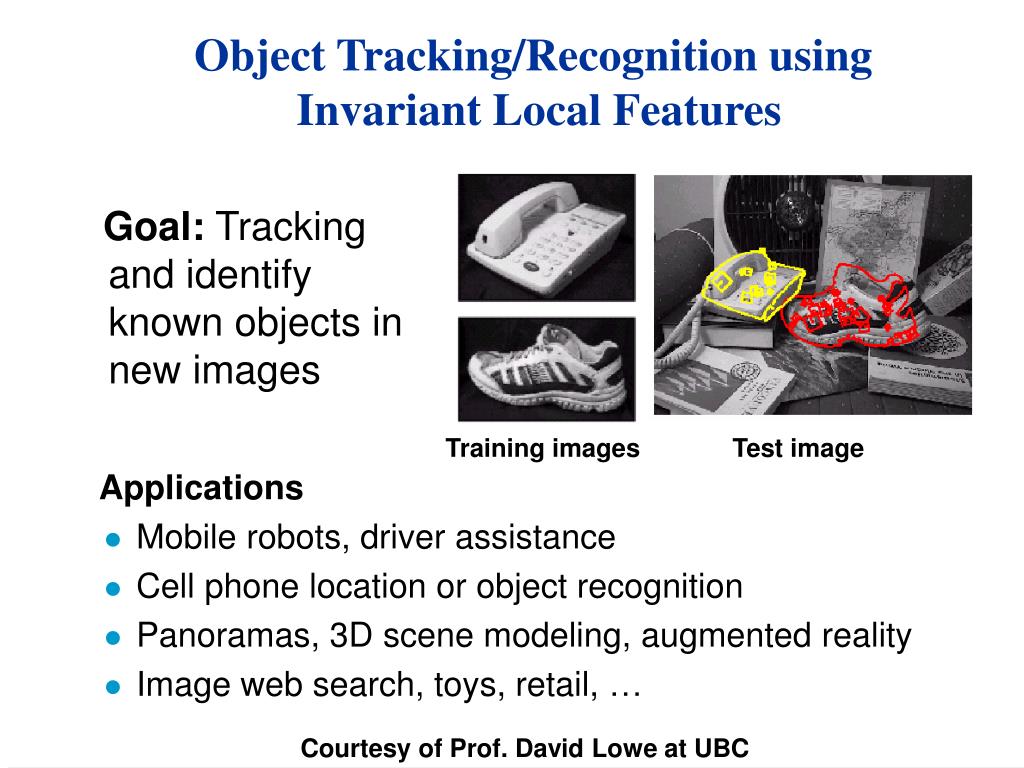
  1. Object Tracking/Recognition using Invariant Local Features Applications • Mobile robots, driver assistance • Cell phone location or object recognition • Panoramas, 3D scene modeling, augmented reality • Image web search, toys, retail, … Goal: Tracking and identify known objects in new images Training images Test image Courtesy of Prof. David Lowe at UBC

  2. Local feature matchingTorr & Murray (93); Zhang, Deriche, Faugeras, Luong (95) • Apply Harris corner detector • Match points by correlating only at corner points • Derive epipolar alignment using robust least-squares

  3. Rotation InvarianceCordelia Schmid & Roger Mohr (97) • Apply Harris corner detector • Use rotational invariants at corner points • However, not scale invariant. Sensitive to viewpoint and illumination change.

  4. Scale-Invariant Local Features (Lowe’2004) • Image content is transformed into local feature coordinates that are invariant to translation, rotation, scale, and other imaging parameters SIFT Features

  5. Advantages of invariant local features • Locality: features are local, so robust to occlusion and clutter (no prior segmentation) • Distinctiveness: individual features can be matched to a large database of objects • Quantity: many features can be generated for even small objects (therefore easy to estimate homography) • Efficiency: close to real-time performance • Extensibility: can easily be extended to wide range of differing feature types, with each adding robustness

  6. Build Scale-Space Pyramid • All scales must be examined to identify scale-invariant features • An efficient function is to compute the Difference of Gaussian (DOG) pyramid (Burt & Adelson, 1983)

  7. Scale space processed one octave at a time

  8. Key point localization • Detect maxima and minima of difference-of-Gaussian in scale space

  9. Select canonical orientation • Create histogram of local gradient directions computed at selected scale • Assign canonical orientation at peak of smoothed histogram • Each key specifies stable 2D coordinates (x, y, scale, orientation)

  10. Example of keypoint detection Threshold on value at DOG peak and on ratio of principle curvatures (Harris approach) • (a) 233x189 image • (b) 832 DOG extrema • (c) 729 left after peak • value threshold • (d) 536 left after testing • ratio of principle • curvatures

  11. SIFT vector formation • Thresholded image gradients are sampled over 16x16 array of locations in scale space • Create array of orientation histograms • 8 orientations x 4x4 histogram array = 128 dimensions

  12. Feature stability to noise • Match features after random change in image scale & orientation, with differing levels of image noise • Find nearest neighbor in database of 30,000 features

  13. Feature stability to affine change • Match features after random change in image scale & orientation, with 2% image noise, and affine distortion • Find nearest neighbor in database of 30,000 features

  14. Distinctiveness of features • Vary size of database of features, with 30 degree affine change, 2% image noise • Measure % correct for single nearest neighbor match

  15. Model verification • Examine all clusters with at least 3 features • Perform least-squares affine fit to model. • Discard outliers and perform top-down check for additional features. • Evaluate probability that match is correct

  16. 3D Object Recognition • Extract outlines with background subtraction

  17. 3D Object Recognition • Only 3 keys are needed for recognition, so extra keys provide robustness • Affine model is no longer as accurate

  18. Recognition under occlusion

  19. Test of illumination invariance • Same image under differing illumination 273 keys verified in final match

  20. Examples of view interpolation

  21. Recognition using View Interpolation

  22. Location recognition

  23. Robot localization results • Joint work with Stephen Se, Jim Little • Map registration: The robot can process 4 frames/sec and localize itself within 5 cm • Global localization: Robot can be turned on and recognize its position anywhere within the map • Closing-the-loop: Drift over long map building sequences can be recognized. Adjustment is performed by aligning submaps.

  24. Robot Localization

  25. Map continuously built over time

  26. Locations of map features in 3D

  27. Sony Aibo • (Evolution Robotics) • SIFT usage: • Recognize • charging • station • Communicate • with visual • cards