Convolution Neural Network CNN
Convolution Neural Network CNN. A tutorial KH Wong. Introduction. Very Popular A high performance Classifier (multi-class) Successful in handwritten optical character OCR recognition, speech recognition, image noise removal etc. Easy to implementation Slow in learning

Convolution Neural Network CNN
E N D
Presentation Transcript
Convolution Neural NetworkCNN A tutorial KH Wong Convolution Neural Network CNN ver. 4.8c
Introduction • Very Popular • A high performance Classifier (multi-class) • Successful in handwritten optical character OCR recognition, speech recognition, image noise removal etc. • Easy to implementation • Slow in learning • Fast in classification Convolution Neural Network CNN ver. 4.8c
Overview of this note • Part 1: Fully connected Back Propagation Neural Networks (BPNN) • Part 1A: feed forward processing • Part 1A: feed backward processing • Part 2: Convolution neural networks (CNN) • Part 2A: feed forward of CNN • Part 2B: feed backward of CNN Convolution Neural Network CNN ver. 4.8c
Part 1 Fully Connected Back Propagation (BP) neural net Convolution Neural Network CNN ver. 4.8c
TheoryFully connected Back Propagation Neural Net (BPNN) • Use many samples to train the weights, so it can be used to classify an unknown input into different classes • Will explain • How to use it after training: forward pass • How to train it: how to train the weights and biases (using forward and backward passes) Convolution Neural Network CNN ver. 4.8c
Training • How to train it: how to train the weights (W) and biases (b) (use forward, backward passes) • Initialize W and b randomly • Iter=1: all_epocks (each is called an epcok) • Forward pass for each output neuron: • Use training samples: Xclass_t : feed forward to find y. • Err=error_function(y-t) • Backward pass: • Find W and b to reduce Err. • Wnew=Wold+W; bnew=bold+b Convolution Neural Network CNN ver. 4.8c
Part 1A Forward pass of Back Propagation Neural Net (BPNN) Recall: Forward pass for each output neuron: -Use training samples: Xclass_t : feed forward to find y. -Err=error_function(y-t) Convolution Neural Network CNN ver. 4.8c
Feed forward of Back Propagation Neural Net (BPNN) • In side each neuron: Convolution Neural Network CNN ver. 4.8c Inputs Output neurons
http://mathworld.wolfram.com/SigmoidFunction.html Sigmod function f(u) and its derivative f’(u) Convolution Neural Network CNN ver. 4.8c http://link.springer.com/chapter/10.1007%2F3-540-59497-3_175#page-1
A single neuron • The neural net can have many layers • In between any neighboring 2 layers, a set of neurons can be found Each Neuron Convolution Neural Network CNN ver. 4.8c
BPNN Forward pass • Forward pass is to find output when an input is given. For example: • Assume we have used N=60,000 images to train a network to recognize c=10 numerals. • When an unknown image is input, the output neuron corresponds to the correct answer will give the highest output level. Input image 10 output neurons for 0,1,2,..,9 Convolution Neural Network CNN ver. 4.8c
The criteria to train a network • Is based on the overall error function Convolution Neural Network CNN ver. 4.8c
Structure of a BP neural network Input layer output layer Convolution Neural Network CNN ver. 4.8c
Architecture (exercise: write formulas for A1(i=4) and A2(k=3) P(j=1) A1 W2(i=1,k=1) W1(j=1,i=1) Neuron k=1 Bias=b2(k=1) Neuron i=1 Bias=b1(i=1) W2(i=2,k=1) W1(j=2,i=1) P(j=2) A2 A1(i=1) W2(i=5,k=1) W1(j=9,i=1) A2(k=2) P(j=9) A5 W1(j=1,i=1) A1(i=1) P(j=1) P(j=2) P(j=3) : : P(j=9) W2(i=1,k=1) W2(i=2,k=1) W1(j=2,i=1) A1(i=2) W2(i=2,k=2) W1(j=3,i=4) W2(i=5,k=3) Output neurons=3 neurons, indexed by k W2=5x3 b2=3x1 A1(i=5) Hidden layer =5 neurons, indexed by i W1=9x5 b1=5x1 W1(j=9,i=5) Input: P=9x1 Indexed by j Convolution Neural Network CNN ver. 4.8c
Answer (exercise: write values for A1(i=4) and A2(k=3) • P=[ 0.7656 0.7344 0.9609 0.9961 0.9141 0.9063 0.0977 0.0938 0.0859] • W1=[ 0.2112 0.1540 -0.0687 -0.0289 0.0720 -0.1666 0.2938 -0.0169 -0.1127] • -b1= 0.1441 • %Find A1(i=4) • A1_i_is_4=1/(1+exp[-(W1*P+b1))] • =0.49 Convolution Neural Network CNN ver. 4.8c
Numerical example for the forward path • Feed forward • Give numbers of x, w b etc Convolution Neural Network CNN ver. 4.8c
Example: a simple BPNN • Number of classes (no. of output neurons)=3 • Input 9 pixels: each input is a 3x3 image • Training samples =3 for each class • Number of hidden layers =1 • Number of neurons in the hidden layer =5 Convolution Neural Network CNN ver. 4.8c
Architecture of the example Input Layer 9x1 pixels output Layer 3x1 Convolution Neural Network CNN ver. 4.8c
Part 1B Backward pass of Back Propagation Neural Net (BPNN) Convolution Neural Network CNN ver. 4.8c
feedback Feed forward Feed backward Convolution Neural Network CNN ver. 4.8c
derivation Convolution Neural Network CNN ver. 4.8c
derivation Convolution Neural Network CNN ver. 4.8c
Numerical example for the feed back pass Convolution Neural Network CNN ver. 4.8c
Procedure • From the last layer (output), find dt-y • Find d, then find w of the whole network • Find iterative (forward- back forward pass) to generate a new set of W, until dW is small • Takes a long time Convolution Neural Network CNN ver. 4.8c
Part 2Convolution Neural Networks Part 2A Feed forward part of cnnff( ) Matlab example http://www.mathworks.com/matlabcentral/fileexchange/38310-deep-learning-toolbox Convolution Neural Network CNN ver. 4.8c
An example optical chartered recognition OCR • Example test_example_CNN.m in http://www.mathworks.com/matlabcentral/fileexchange/38310-deep-learning-toolbox • Based on a data base (mnist_uint8, from http://yann.lecun.com/exdb/mnist/) • 60,000 training examples (28x28 pixels each) • 10,000 testing samples (a different dat.2set) • After training , given an unknown image, it will tell whether it is 0, or 1 ,..,9 etc. • Recognition rate 11% use 1 epoch (training 200seconds) • Recognition rate 1.2% use 100 epochs (hours of training) http://andrew.gibiansky.com/blog/machine-learning/k-nearest-neighbors-simplest-machine-learning/ Convolution Neural Network CNN ver. 4.8c
Overview ofTest_example_CNN.m • Read data base • Part I: • cnnsetup.m • Layer 1: input layer (do nothing) • Layer 2 convolution(conv.) Layer, output maps=6, kernel size=5x5 • Layer 3 sub-sample (subs.) Layer, scale=2 • Layer 4 conv. Layer, output maps =12, kernel size=5x5 • Layer 5 subs. Layer (output layer), scale =2 • Part 2: • cnntrain.m % train wedihgts using 60,000 samples • cnnff( ) % CNN feed forward • cnndb( ) % CNN feed back to train weighted in kernels • cnnapplygrads( ) % update weights • cnntest.m % test the system using 10000 samples and show error rate Convolution Neural Network CNN ver. 4.8c
Architecture Layer 34: 12 conv. Maps (C) InputMaps=6 OutputMaps=12 Fan_in= 6x52=150 Fan_out= 12x52=300 Each output neuron corresponds to a character (0,1,2,..,9 etc.) Layer 12: 6 conv.Maps (C) InputMaps=6 OutputMaps=6 Fan_in=52=25 Fan_out=6x52=150 Layer 23: 6 sub-sample Map (S) InputMaps=6 OutputMaps=12 Layer 45: 12 sub-sample Map (S) InputMaps=12 OutputMaps=12 Layer 1: One input (I) Layer 1: Image Input 1x28x28 Layer 2: 6x24x24 Layer 3: 6x12x12 Layer 4: 12x8x8 Layer 5: 12x4x4 Conv. Kernel =5x5 Subs Kernel =5x5 Conv. 2x2 Subs I=input C=Conv.=convolution S=Subs=sub sampling 2x2 10 Convolution Neural Network CNN ver. 4.8c
Cnnff.mconvolution neural networks feed forward • This is the feed forward part • Assume all the weights are initialized or calculated, we show how to get the output from inputs. Convolution Neural Network CNN ver. 4.8c
Layer 12: Layer 12: 6 conv.Maps (C) InputMaps=6 OutputMaps=6 Fan_in=52=25 Fan_out=6x52=150 Layer 1: One input (I) • Convolute layer 1 with different kernels (map_index1=1,2,.,6) and produce 6 output maps • Inputs : • input layer 1, a 28x28 image • 6 different kernels : k(1),.,,,k(6) , each k is 5x5, K are dendrites of neurons • Output : 6 output maps each 24x24 • Algorithm • For(map_index=1:6) • { • layer_2(map_index)= • I*k(map_index)valid • } • Discussion • Valid means only consider overlapped areas, so if layer 1 is 28x28, kernel is 5x5 each, each output map is 24x24 • In Matlab > use convn(I,k,’valid’) • Example: • I=rand(28,28) • k=rand(5,5) • size(convn(I,k,’valid’)) • > ans • > 24 24 Layer 1: Image Input (i) 1x28x28 Layer 2(c): 6x24x24 Map_index= 1 2 : 6 i Conv.*K(1) Kernel =5x5 Conv.*K(6) j 2x2 I=input C=Conv.=convolution S=Subs=sub sampling Convolution Neural Network CNN ver. 4.8c
Sub-sample layer 2 to layer 3 • Inputs : • 6 maps of layer 2, each is 24x24 • Output : 6 maps of layer 3, each is 12 x12 • Algorithm • For(map_index=1:6) • { • For each input map, calculate the average of 2x2 pixels and the result is saved in output maps. • Hence resolution is reduced from 24x24 to 12x12 • } • Discussion Layer 23: Layer 23: 6 sub-sample Map (S) InputMaps=6 OutputMaps=12 Layer 2 (c): 6x24x24 Layer 3 (s): 6x12x12 Map_index= 1 2 : 6 Subs 2x2 Convolution Neural Network CNN ver. 4.8c
Conv. layer 3 with kernels to produce layer 4 • Inputs : • 6 maps of layer3(L3{i=1:6}), each is 12x12 • Kernel set: totally 6x12 kernels, each is 5x5,i.e. • K{i=1:6}{j=1:12}, each K{i}{j} is 5x5 • 12 bias{j=1:12} in this layer, each is a scalar • Output : 12 maps of layer4(L4{j=1:12}), each is 8x8 • Algorithm • for(j=1:12) • {for (i=1:6) • {clear z, i.e. z=0; • z=z+covn (L3{i}, k{i}{j},’valid’)] %z is 8x8 • } • L4{j}=sigm(z+bais{j}) %L4{j} is 8x8 • } • function X = sigm(P) • X = 1./(1+exp(-P)); • End • Discussion • Normalization? Layer 34: Layer 34: 12 conv. Maps (C) InputMaps=6 OutputMaps=12 Fan_in= 6x52=150 Fan_out= 12x52=300 Layer3 L3(s): 6x12x12 Layer 4(c): 12x8x8 net.layers{l}.a{j} Index=i=1:6 Index=j=1:12 : Kernel =5x5 Convolution Neural Network CNN ver. 4.8c
Subsample layer 4 to layer 5 • Inputs : • 12 maps of layer4(L4{i=1:12}), each is 12x8x8 • Output : 12 maps of layer5(L5{j=1:12}), each is 4x4 • Algorithm • Sub sample each 2x2 pixel window in L4 to a pixel in L5 • Discussion • Normalization? Layer 45 Layer 45: 12 sub-sample Map (S) InputMaps=12 OutputMaps=12 Layer 4: 12x8x8 Layer 5: 12x4x4 Subs 2x2 10 Convolution Neural Network CNN ver. 4.8c
Subsample layer 4 to layer 5 • Inputs : • 12 maps of layer5(L5{i=1:12}), each is 4x4, so L5 has 192 pixels in total • Output layer weights: Net.ffW{m=1:10}{p=1:192}, total number of weights is 192 • Output : 10 output neurons (net.o{m=1:10}) • Algorithm • For m=1:10%each output neuron • {clear net.fv • net.fv=Net.ffW{m}{all 192 weight}.*L5(all corresponding 192 pixels) • net.o{m}=sign(net.fv + bias) • } • Discussion Layer 5output Layer 45: 12 sub-sample Map (S) InputMaps=12 OutputMaps=12 Totally 192 weights for each output neuron Each output neuron corresponds to a character (0,1,2,..,9 etc.) net.o{m=1:10} Layer 5 (L5{j=1:12}: 12x4x4=192 Totally 192 pixels : : Same for each output neuron 10 Convolution Neural Network CNN ver. 4.8c
Part 2B Back propagation part cnnbp( ) cnnapplyweight( ) Convolution Neural Network CNN ver. 4.8c
cnnbp( )overview (output back to layer 5 Convolution Neural Network CNN ver. 4.8c Ref: See http://en.wikipedia.org/wiki/Backpropagation
Layer 5 to 4 • Expand 1x1 to 2x2 Convolution Neural Network CNN ver. 4.8c
Layer 4 to 3 • Rotated convolution • Find dE/dx at layer 3 Convolution Neural Network CNN ver. 4.8c
Layer 3 to 2 • Expand 1x1 to 2x2 Convolution Neural Network CNN ver. 4.8c
Calculate gradient • From later 2 to layer 3 • From later 3 to layer 4 • Net.ffW • Net.ffb found Convolution Neural Network CNN ver. 4.8c
Details of calc gradients • % part % reshape feature vector deltas into output map style • L4(c) run expand only • L3(s) run conv (rot180, fill), found d • L2(c) run expand only • %Part %% calc gradients • L2(c) run conv (valid), found dk and db • L3(s) not run here • L4(c) run conv(valid), found dk and db • Done , found these for the output layer L5: • net.dffW = net.od * (net.fv)' / size(net.od, 2); • net.dffb = mean(net.od, 2); Convolution Neural Network CNN ver. 4.8c
cnnapplygrads(net, opts) • For the convolution layers, L2, L4 • From k and dk find new k (weights) • From b and db find new b (bias) • For the output layer L5 • net.ffW = net.ffW - opts.alpha * net.dffW; • net.ffb = net.ffb - opts.alpha * net.dffb; • opts.alpha is to adjust learning rate Convolution Neural Network CNN ver. 4.8c
appendix Convolution Neural Network CNN ver. 4.8c
Architecture Layer 34: 12 conv. Maps (C) InputMaps=6 OutputMaps=12 Fan_in= 6x52=150 Fan_out= 12x52=300 Each output neuron corresponds to a character (0,1,2,..,9 etc.) Layer 12: 6 conv.Maps (C) InputMaps=6 OutputMaps=6 Fan_in=52=25 Fan_out=6x52=150 Layer 23: 6 sub-sample Map (S) InputMaps=6 OutputMaps=12 Layer 45: 12 sub-sample Map (S) InputMaps=12 OutputMaps=12 Layer 1: One input (I) Layer 1: Image Input 1x28x28 Layer 2: 6x24x24 Layer 3: 6x12x12 Layer 4: 12x8x8 Layer 5: 12x4x4 i u v Conv. Kernel =5x5 Subs Kernel =5x5 Conv. 2x2 I=input C=Conv.=convolution S=Subs=sub sampling Subs 2x2 10 Convolution Neural Network CNN ver. 4.8c j
A single neuron • The neural net has many layers • In between any neighboring 2 layers, a set of neurons can be found Each Neuron Convolution Neural Network CNN ver. 4.8c
Derivation • dE/dW=changes at layer l+1 by changes in layer l • At output layer L • dE/db=d • E=f(wx+b) • dE/db=d Convolution Neural Network CNN ver. 4.8c
References • Wiki • http://en.wikipedia.org/wiki/Convolutional_neural_network • http://en.wikipedia.org/wiki/Backpropagation • Matlab programs • Neural Network for pattern recognition- Tutorial http://www.mathworks.com/matlabcentral/fileexchange/19997-neural-network-for-pattern-recognition-tutorial • CNN Matlab example http://www.mathworks.com/matlabcentral/fileexchange/38310-deep-learning-toolbox Convolution Neural Network CNN ver. 4.8c