Download
1 / 39
390 likes | 408 Vues
Explore the conservation of mass, salt, heat, momentum equations, and forces governing ocean motion. Dive into pressure gradients, Coriolis, gravity, and more.

E N D
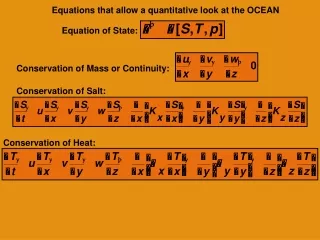
Conservation of Mass or Continuity: Conservation of Salt: Conservation of Heat: Equation of State: Equations that allow a quantitative look at the OCEAN
Conservation of Momentum (Equations of Motion) Newton’s Second Law: as they describe changes of momentum in time per unit mass Conservation of momentum
z x Circulación típica en un fiordo
z x Aceleraciones
z x Gradiente de presión Debido a la pendiente del nivel del mar (barotrópico) Debido al gradiente de densidad (baroclínico)
z x Fricción Debida a gradientes verticales de velocidad (divergencia del flujo de momentum)
z x Coriolis Debido a la rotación de la Tierra; proporcional a la velocidad
z x Balance de momentum
Forces per unit mass that produce accelerations in the ocean: Pressure gradient + Coriolis + gravity + friction + tides Pressure gradient: Barotropic and Baroclinic Coriolis: Only in the horizontal Gravity: Only in the vertical Friction: Surface, bottom, internal Tides: Boundary condition REMEMBER, these are FORCES PER UNIT MASS
Pressure gradient + gravity + Coriolis + friction + tides Pressure gradient: Barotropic and Baroclinic Coriolis: Only in the horizontal Gravity: Only in the vertical Friction: Surface, bottom, internal Tides: Boundary condition REMEMBER, these are FORCES PER UNIT MASS
Net Force in ‘x’ = Net Force per unit mass in ‘x’ = Total pressure force/unit mass on every face of the fluid element is:
Pressure of water column at 1 (hydrostatic pressure) : Pressure Gradient Pressure Gradient Force Hydrostatic pressure at 2 : Pressure gradient force caused by sea level tilt: BAROTROPIC PRESSURE GRADIENT Illustrate pressure gradient force in the ocean Pressure Gradient? z 1 2
Aporte aproximado por lluvia: 2000 mm por año area superficial: 350 km por 10 km = 3.5x10⁹ m2 200 m3/s Aporte aproximado por ríos: 1000 m3/s Milliman et al. (1995) Dirección Meteorológica de Chile Descarga de Agua Dulce Precipitación pluvial y Ríos
Pressure gradient + Coriolis + gravity + friction + tides Pressure gradient: Barotropic and Baroclinic Coriolis: Only in the horizontal Gravity: Only in the vertical Friction: Surface, bottom, internal Tides: Boundary condition REMEMBER, these are FORCES PER UNIT MASS
Acceleration due to Earth’s Rotation Remember cross product of two vectors: and
, Now, let us consider the velocity of a fixed particle on a rotating body at the position The body, for example the earth, rotates at a rate To an observer from space (us): This gives an operator that relates a fixed frame in space (inertial) to a moving object on a rotating frame on Earth (non-inertial)
0 Acceleration of a particle on a rotating Earth with respect to an observer in space Coriolis Centripetal This operator is used to obtain the acceleration of a particle in a reference frame on the rotating earth with respect to a fixed frame in space
Coriolis Acceleration Ch Cv The equations of conservation of momentum, up to now look like this:
Making: f is the Coriolis parameter • This can be simplified with two assumptions: • Weak vertical velocities in the ocean (w << v, u) • Vertical component is ~5 orders of magnitude < acceleration due to gravity
Eastward flow will be deflected to the south Northward flow will be deflected to the east f increases with latitude fis negative in the southern hemisphere
Pressure gradient + Coriolis + gravity + friction + tides Pressure gradient: Barotropic and Baroclinic Coriolis: Only in the horizontal Gravity: Only in the vertical Friction: Surface, bottom, internal Tides: Boundary condition
Pressure gradient + Coriolis + gravity + friction + tides Pressure gradient: Barotropic and Baroclinic Coriolis: Only in the horizontal Gravity: Only in the vertical Friction: Surface, bottom, internal Tides: Boundary condition REMEMBER, these are FORCES PER UNIT MASS
g has a weak variation with latitude because of the magnitude of the centrifugal acceleration g is maximum at the poles and minimum at the equator (because of both r and lamda) Centripetal acceleration and gravity
Variation in g with latitude is ~ 0.5%, so for practical purposes, g =9.80 m/s2
Friction (wind stress) z W Vertical Shears (vertical gradients) u
Friction (bottom stress) Vertical Shears (vertical gradients) z u bottom
Friction (internal stress) Vertical Shears (vertical gradients) z u1 u2 Flux of momentum from regions of fast flow to regions of slow flow
Shear stress is proportional to the rate of shear normal to which the stress is exerted at molecular scales µ is the molecular dynamic viscosity = 10-3 kg m-1 s-1 for water is a property of the fluid Shear stress has units of kg m-1 s-1 m s-1 m-1 = kg m-1 s-2 or force per unit area or pressure: kg m s-2 m-2 = kg m-1 s-2
becomes: If viscosity is constant, And up to now, the equations of motion look like: These are the Navier-Stokes equations Presuppose laminar flow!
Reynolds Number Inertial to viscous: Compare non-linear (advective) terms to molecular friction Flow is laminar when Re < 1000 Flow is transition to turbulence when 100 < Re < 105 to 106 Flow is turbulent when Re > 106, unless the fluid is stratified
Low Re High Re
Consider an oceanic flow where U = 0.1 m/s; L = 10 km; kinematic viscosity = 10-6 m2/s Is friction negligible in the ocean?
Frictional stresses from turbulence are not negligible but molecular friction is negligible at scales > a few m. • - Use these properties of turbulent flows in the Navier Stokes equations • The only terms that have products of fluctuations are the advection terms • All other terms remain the same, e.g.,
0 are the Reynolds stresses arise from advective (non-linear or inertial) terms
This relation (fluctuating part of turbulent flow to the mean turbulent flow) is called a turbulence closure The proportionality constants (Ax, Ay, Az) are the eddy (or turbulent) viscosities and are a property of the flow (vary in space and time)
Ax, Ay oscillate between 101 and 105m2/s Azoscillates between 10-5 and 10-1m2/s Az<< Ax, Ay but frictional forces in vertical are typically stronger eddy viscosities are up to 1011 times > molecular viscosities