

SlideServe
Menu
Préférences
© SlideServe · v2026

Kruskal Wallis

khuyen avatar
10 diapositives · 660 Views · Sep 30, 2014

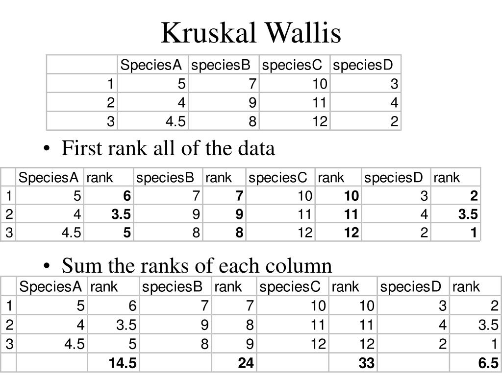
Kruskal Wallis. First rank all of the data Sum the ranks of each column. Kruskal Wallis. Find the square of each R Ra 2 = 210.3 Rb 2 =576 Rc 2 =1089 Rd 2 =42.25 H = 12 (Sum [R 2 /(number in column ]) – 3(N +1) N(N +1) H= {12/156(70.1 +192+363+14.08)} -39 H=10.2
Kruskal Wallis - slide 1
01 / 10Kruskal Wallis
1 / 17

Télécharger la présentation

Kruskal Wallis
Une image / un lien ci-dessous est fourni (tel quel) pour télécharger la présentation

Politique de téléchargement : le contenu du site vous est fourni TEL QUEL pour votre information et votre usage personnel ; il ne peut être vendu, concédé sous licence ni partagé sur d’autres sites sans l’accord de son auteur.Le contenu vous est fourni TEL QUEL, pour votre information et votre usage personnel uniquement. Téléchargez la présentation en cliquant sur ce lien. Lors du téléchargement, si vous ne parvenez pas à télécharger une présentation, l’éditeur a peut-être supprimé le fichier de son serveur.Pendant le téléchargement, si vous ne parvenez pas à obtenir une présentation, le fichier a peut-être été supprimé par l’éditeur.

F I N

Plus de contenu associé

Transcription de la présentation
  1. Kruskal Wallis • First rank all of the data • Sum the ranks of each column

  2. Kruskal Wallis • Find the square of each R • Ra2=210.3 Rb2=576 Rc2=1089 Rd2=42.25 • H = 12 (Sum [R 2/(number in column]) – 3(N +1) N(N +1) • H= {12/156(70.1+192+363+14.08)} -39 • H=10.2 • Df=(#of columns)-1 • Use the critical value from the chi square table df3=7.82 • If value is greater than critical than there are differences between groups

  3. Kruskal Wallis multiple comparisons • |Ra-Rb| >= Z alpha/k(k-1)sqr.root[N(N+1)/12{1/Na+1/Nb}] • |Ra-Rb| = 9.5 • Z alpha/k(k-1) Is found in the Z distribution • Use table (table Aii, pg320) • C=k(k-1)/2=6 Z=2.638 • 9.5>7.76 • Repeat procedure for all six combinations

  4. Chicken Lab Statistics

  5. Basic stats • Event behaviors- Frequency per unit time • State behaviors – • average duration (use any of the compairisons we already taught you) • Duration percentage (useful for when the duration of observation is not always the same, no good statistic) v

  6. Non Ratio data • Frequency data is not ratio data • Therefore you cannot use any of the tests we have discussed that are based on a normal distribution • Frequency data utilzes a poisson distribution and hypothesis are tested using a chi square statistic.

  7. Goodness of fit test • Different levels of a single variable • Comparing the frequency of behavior of one chick across days X2 = Sum (observed frequency – Expected frequency)2 Expected frequency Expected frequencies = assume equal distribution of frequencies Degrees of freedom - # categories - 1

  8. Goodness of fit • X2 = (39-25)2/25 + (15-25)2/25 + (28-25)2/25 + (18-25)2/25 • = 196/25 + 100/25 + 9/25 +49/25 • =14.96 • Critical values are found in the table on pg 153 of Brown and Downhower • If your value exceeds the table value (7.8) than we can conclude that the frequencies are not evenly distributed across categories

  9. Test of independence • Test based on two categorical variables • Tests that the two categories are not related in any way • Comparing the frequencies of your two different chicks across days X2 = Sum (observed frequency – Expected frequency)2 Expected frequency Degrees of freedom – (# rows – 1)(#columns –1)

  10. Test of independence • Expected frequency = row total x column total N X2 = 9 + 1 + 1 + 9 + 9 + 1 + 1 + 9 = 40 Df = 3 crit value = 7.8 Therefore there is a significant difference in the development of the two groups of chickens