Download

1 / 22
230 likes | 471 Vues
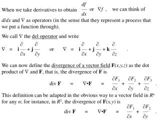
df — or f , we can think of dx. When we take derivatives to obtain. d / dx and as operators (in the sense that they represent a process that we put a function through). We call the del operator and write. = i — + j — or x y.

E N D
df — or f , we can think of dx When we take derivatives to obtain d/dx and as operators (in the sense that they represent a process that we put a function through). We call the del operator and write = i — + j — or x y = i — + j — + k — . x y z We can now define the divergence of a vector fieldF(x,y,z) as the dot product of and F, that is, the divergence of F is F1 F2 F3 div F = •F = — + — + — . x y z This definition can be adapted in the obvious way to a vector field in Rn for any n; for instance, in R2, the divergence of F(x,y) is F1 F2 div F = •F = — + — . x y
If a vector field in R3 represents the velocity field of a gas or fluid, the divergence can be interpreted as the rate of expansion per unit volume, while such a vector field in R2 can be interpreted as the rate of expansion per unit area. Consider the vector field described by F(x,y) = xi + yj . The flow lines point If the flow lines are those of a gas, then the gas is as it moves away from the origin. Consequently, we should expect that div F > 0. We verify this by observing that away from the origin. expanding div F = 1 + 1 = 2 > 0. Consider the vector field described by F(x,y) = – xi – yj . The flow lines point If the flow lines are those of a gas, then the gas is as it moves toward the origin. Consequently, we should expect that div F < 0. We verify this by observing that toward the origin. compressing div F = – 1 – 1 = – 2 < 0
Consider the vector field described by F(x,y) = – yi + xj . In a previous example, we found that the flow lines are If the flow lines are those of a gas, then the gas is Consequently, we should expect that div F = 0. We verify this by observing that concentric, counterclockwise circles around the origin. neither compressing nor expanding as it moves around the origin. div F = 0 + 0 = 0. Consider the vector field described by F(x,y) = x2yi – xj . It is not easy to intuit what the divergence will be. By obtaining div F = , we find that 2xy + 0 = 2xy the divergence is not the same at all points in the vector field. (compression) (expansion) (expansion) (compression)
We define the curl of a vector fieldF(x,y,z) as the cross product of and F, that is, the curl of F is F3 F2 F1 F3 F2 F1 curl F = F = ( — – — )i + ( — – — )j + ( — – — )k . y z z x x y Curl is an operator defined only in R3, whereas divergence is an operator defined in Rn for any n. If F(x,y,z) = – yi + xj + zk , then curl F = 2k . If F(x,y,z) = x2yi – xzj + yz2k , then curl F = (z2+x)i + 0j + (– z – x2)k .
Let us find the curl for a vector field which describes motion of points in a rotating body with axis of rotation along the z axis; the value of the vector field at each point is the velocity vector v at that point. We let position vector of a point on the rotating object r = xi + yj + zk = v = velocity vector of a point on the rotating object (i.e., the vector field) = angular velocity of a point on the rotating object x2 + y2(e.g., speed doubles if distance to z axis is doubled.) ||v|| = xy plane k v r = position vector of a point on the rotating object Observe that v is in the direction of kr = k(xi + yj + zk) = – yi + xj v = – yi + xj curl v = 2k . If a vector field F represents the flow of a fluid, then we see that curl F at a point has a magnitude of twice the angular velocity vector of a rigid rotation in the direction of the axis of rotation; if (curl F) = 0 = 0i + 0j + 0k at a point, then the fluid is free from rigid rotations (i.e., whirlpools) at that point.
Consider the vector field described by y x F(x,y,z) = ——— i – ——— j . x2 + y2x2 + y2 Using results from a previous example, we find that for any plane parallel to the xy plane, the flow lines form concentric, clockwise circles around the origin, with velocity becoming larger closer to the origin. curl F = (0 – 0)i + (0 – 0)j + 0k = 0. When (curl F) = 0 for a fluid, then a sufficiently small object (such as a paddle wheel) will not rotate as it moves with the fluid (even though the object may be “rotating” around a point with the fluid flow). Such a vector field is called irrotational.
Suppose V is a vector field from R3 to R3, and V = f, where f is a function with continuous partial derivatives of at least the second order, i.e., V is a gradient vector field. Then, curl V = V = (f) = (fxi + fyj + fzk) = (fzy – fyz)i + (fxz – fzx)j + (fyx – fxy)k = 0i + 0j + 0k = 0 . Consequently, if (curl V) 0, then V cannot be a gradient vector field. It can be shown that for vector fields V with continuous component functions, V is a gradient vector field if and only if (curl V) =0. Is the vector field described by y x F(x,y,z) = ——— i – ——— j a gradient vector field? x2 + y2x2 + y2 Since we have previously seen that (curl F) = 0, then we know that F is a gradient vector field. (In fact, F = f, where f(x,y,z) = Arctan(x/y).)
Could it be possible that the vector field described by F(x,y,z) = yi– xj is a gradient vector field? Since curl F = (0 – 0)i + (0 – 0)j + (– 1 – 1)k = – 2k , then F cannot be a gradient vector field. Note that if F = P(x,y)i + Q(x,y)j is a vector field in R2, then F can be regarded as a vector field in R3 by letting F = P(x,y)i + Q(x,y)j + 0k . (0 – 0)i + (0 – 0)j + (Qx– Py)k = (Qx– Py)k . The function Qx– Py is called the scalar curl of F. We then have that curl F = Consider the vector field described by F(x,y) = yi– x2j. The scalar curl is – 2x – 1 .
Suppose V = P(x,y,z)i + Q(x,y,z)j + R(x,y,z)k is a vector field with each of the three component functions having continuous partial derivatives of at least the second order. Then, div (curl V) = •(V) = •[( )i + ( )j + ( )k] = Ry – Qz Pz – Rx Qx – Py ( ) + ( ) + ( ) = Ryx– Qzx Pzy– Rxy Qxz– Pyz 0 Consequently, if (div F) 0, then F cannot be the curl of any vector field. It can be shown that for vector fields F with continuous component functions, F is the curl of another vector field if and only if div(F) = 0. Can F(x,y,z) = xi + yj + zk possibly be the curl of another vector field? Since div F = 1 + 1 + 1 = 3 0 , then F is not the curl of any vector field. Can F(x,y,z) = yi + zj + xk possibly be the curl of another vector field? Since div F = 0 + 0 + 0 = 0 , then F is the curl of another vector field.
Consider again the definition of (div V) = •V, and suppose that V = f, where f is a function with continuous partial derivatives of at least the second order, i.e., V is a gradient vector field. Then, we may write 2f 2f 2f — + — + — . x2 y2 z2 (div V) = •V = •(f) = 2f = The operator 2 is called the Laplace operator. Find 2f for f(x,y,z) = 1 / (x2+y2+z2)1/2. fx = fxx = fy = fyy = fz =fzz = – x / (x2+y2+z2)3/2 3x2 / (x2+y2+z2)5/2 – 1 / (x2+y2+z2)3/2 – y / (x2+y2+z2)3/2 3y2 / (x2+y2+z2)5/2 – 1 / (x2+y2+z2)3/2 – z / (x2+y2+z2)3/2 3z2 / (x2+y2+z2)5/2 – 1 / (x2+y2+z2)3/2 2f = 0
Page 306 displays several vector identities. 1) (f+g) = (fx+gx)i + (fy+gy)j + (fz+gz)k = (fxi + fyj + fzk) + (gxi + gyj + gzk) = f + g 2) (cf) = (cfx)i + (cfy)j + (cfz)k = c(fxi + fyj + fzk) = cf 3) (fg) = (fxg+fgx)i + (fyg+fgy)j + (fzg+fgz)k = (fxgi + fygj + fzgk) + (fgxi + fgyj + fgzk) = g(fxi + fyj + fzk) + f(gxi + gyj + gzk) = gf + fg = fg + gf 4) (f / g) = [(fxg–fgx) / g2]i + [(fyg–fgy) / g2]j + [(fzg–fgz) / g2]k = (1/g2)[(fxg–fgx)i + (fyg–fgy)j + (fzg–fgz)k] = (1/g2)[(fxgi + fygj + fzgk) – (fgxi + fgyj + fgzk)] = (gf – fg) / g2 (at points where g 0)
div(F+G) = •(F+G) = —(F1+G1) + —(F2+G2) + —(F3+G3) = x y z 5) F1 G1 F2 G2 F3 G3 — + — + — + — + — + — = x x y y z z F1 F2 F3 G1 G2 G3 — + — + — + — + — + — = x y z x y z •F + •G = (div F) + (div G)
6) curl(F+G) = (F+G) = [ —(F3+G3) – —(F2+G2) ] i + y z [ —(F1+G1) – —(F3+G3) ] j + z x [ —(F2+G2) – —(F1+G1) ] k = x y F3 G3 F2 G2 [ — + — – — – — ] i + y y z z [ ] j + [ ] k =
F3 F2 G3 G2 [ — – — + — – — ] i + y z y z [ ] j + [ ] k = F3 F2 [ — – — ] i + [ ] j + [ ] k + y z G3 G2 [ — – — ] i + [ ] j + [ ] k = y z F + G = curl(F) + curl(G)
div(fF) = •(fF) = —(fF1) + —(fF2) + —(fF3) = x y z 7) F1 f F2 f F3 f f — + — F1 + f — + — F2 + f — + — F3 = x x y y z z F1 F2 F3 f f f f — + f — + f — + F1 — + F2 — + F3 — = x y z x y z f•F + F•f = f(div F) + F•f
8) div(FG) = •(FG) = •[(F2G3–F3G2)i + (F3G1–F1G3)j + (F1G2–F2G1)k] = —(F2G3–F3G2) + —(F3G1–F1G3) + —(F1G2–F2G1) = x y z F2 G3 F3 G2 ( — G3 + F2 — ) – ( — G2 + F3— ) + x x x x ( ) – ( ) + ( ) – ( ) =
F3 F2 F1 F3 F2 F1 G1 ( — – — ) + G2( — – — ) + G3( — – — ) y z z x x y – ( ) – ( ) – ( ) = G•(F) – F•(G) = G•(curl F) – F•(curl G)
9) div (curl F) = 0 (proven in an earlier class) Suppose V = P(x,y,z)i + Q(x,y,z)j + R(x,y,z)k is a vector field with each of the three component functions having continuous partial derivatives of at least the second order. Then, div (curl V) = •(V) = •[( )i + ( )j + ( )k] = Ry – Qz Pz – Rx Qx – Py ( ) + ( ) + ( ) = Ryx– Qzx Pzy– Rxy Qxz– Pyz 0 10) curl(fF) = (fF) = [—(fF3) – —(fF2) ]i + [—(fF1) – —(fF3) ]j + [—(fF2) – —(fF1) ]k = y z z x x y F3 f F2 f [( f — + — F3 ) – (f — + — F2 ) ]i + y y z z [ ( ) – ( ) ]j+ [ ( ) – ( ) ]k=
F3 F2 F1 F3 F2 F1 f ( — – — )i + f( — – — )j + f( — – — )k + y z z x x y ( )i+ ( )j + ( )k= f curl F+ (f)F (f)(F) + (f)F=
11) curl(f) = curl(fxi + fyj + fzk) = fz fyfx fz fy fx ( — – — )i + ( — – — )j + ( — – — )k = y z z x x y (fyz– fyz)i + (fxz– fxz)j + (fxy–fxy)k = 0 (proven in an earlier class) 2 2 2 2(fg) = —(fg) + —(fg) + —(fg) = x2 y2 z2 12) —(fxg+fgx) + —(fyg+fgy) + —(fzg+fgz) = x y z (fxxg+fxgx+fxgx+fgxx) + (fyyg+fygy+fygy+fgyy) + (fzzg+fzgz+fzgz+fgzz) = (fgxx+fgyy+fgzz) + (fxxg+fyyg+fzzg) + (2fxgx+2fygy+2fzgz) = f2g + g2f + 2(f • g)
The easy way to prove #13 is to use #8 which has been already proven: div(f g) = g• (curl(f)) – f•(curl(g)) = g• 0– f•0 = 0– 0 = 0 13) div(f g) = div[ (fygz– fzgy)i + (fzgx– fxgz)j + (fxgy– fygx)k ] = —(fygz– fzgy) + —(fzgx– fxgz) + —(fxgy– fygx) = x y z (fyxgz + fygzx– fzxgy – fzgyx) + (fzygx + fzgxy– fxygz– fxgyz) + (fxzgy + fxgyz– fyzgx – fygxz) = 0
14) div(fg –gf) = div[ (fgxi + fgyj + fgzk) – (gfxi + gfyj + gfzk) ] = div[ (fgx– gfx)i + (fgy– gfy)j + (fgz– gfz)k ] = —(fgx– gfx) + —(fgy– gfy) + —(fgz– gfz) = x y z (fxgx + fgxx– gxfx – gfxx) + (fygy + fgyy– gyfy – gfyy) + (fzgz + fgzz– gzfz – gfzz) = (fgxx– gfxx) + (fgyy– gfyy) + (fgzz– gfzz) = fgxx + fgyy + fgzz– (gfxx +gfyy + gfzz) = f2g –g2f