Curves and Surfaces
Curves and Surfaces. CSE3AGR - Paul Taylor 2009. Polynomials of Degree n. Degree is equal to the highest exponent of a term. Higher exponents result in more and more possible curves A degree n Polynomial can represent all curves that can be represented by ANY <n polynomials. Linear x.

Curves and Surfaces
E N D
Presentation Transcript
Curves and Surfaces CSE3AGR - Paul Taylor 2009
Polynomials of Degree n • Degree is equal to the highest exponent of a term. • Higher exponents result in more and more possible curves • A degree n Polynomial can represent all curves that can be represented by ANY <n polynomials.
Linear x • https://harmon-middle-school.wikispaces.com/file/view/Graph.psd.jpg
Quadratic x2 • http://www.nipissingu.ca/calculus/tutorials/quadratics.html
Cubic x3 • http://en.wikipedia.org/wiki/File:Polynomialdeg3.svg
Quartic x4 • http://en.wikipedia.org/wiki/Quartic_equation
Quintic x5 • http://en.wikipedia.org/wiki/File:Polynomialdeg5.png
Representin’ Explicit Implicit Parametric
Explicit • Solve the new state of the system based on its previous state
Explicit • Just like in High-School • One variable is dependant, the other Independant • Y = f(x) • Eg: y = x2 • Sometimes the function is invertertable • X = g(y) • Eg: x = y(1/2)
Problems Explicit Functions can fail on specific orientations!!! A Simple Line y = mx + c A Vertical Line all values of Y will only exist for 1 value of x
A Circle • A circle is a curve with a constant rate of bending • The closest we can get using an explicit rep: • Y = (r2 + x2) • Y = -(r2 - x2) • Given 0 ≤ |x| ≤ r
3D Explicit Functions • We need two functions to represent a curve in 3D. • Given X we have 2 dependant variables: • Y = f(x) • Z = f(x)
Explicit Surfaces • A Surface requires two independent variables Z = f( x, y)
Pros & Cons of Explicits • Mathematically Perfect • But Mathematicians never had to render an infinite value!!! • A Good use of explicits is intersection testing • Did the ray Intersect the Circle? • r = (y2 + x2) • A sphere • r = -(z2 + y2 + x2)
Implicit • Solve the new state of the system based on its previous state and the current state
Implicits • F( x, y) = 0 In 2 Dimensions: A Line: Ax + by + c = 0 A Circle: x2 + y2 – r2 = 0
Pros & Cons of Implicits Also very useful for membership testing. Eg: Does (3,7) belong to the curve? Curves must be described as the intersection of two curved surfaces. :-S Quadrics are a quadratic polynomial type of surface, which can be represented implicitly. - Quadrics are also simple to intersect with lines
Parametric Equations These guys are pretty much the staple diet of Cg curves! Basically they are created using three related explicit functions
Pros & Cons of Parametrics • Always solvable! • Great for cheating with pre-calculated Basis Matrices
Joining Cubics • Continuity is what we need!! • We have two levels of continuity • Geometric and Parametric • Geometric is simply ‘it looks pretty good!’ • Parametric is where the continuity is perfectly defined. • Parametric Continuity infers geometric Continuity • This is not transient • We can create Geometric Continuity by slacking off on Parametric Equations
3 Levels of Cohesion • Level 0 • Both curves share a point in space • Level 1 • Both curves share the point in space and have tangents (Gradients) that point in the same direction. (matching Velocity in time based visualisation) • Level 2 • Both curves share the point in space and have tangents (Gradients) that point in the same direction with the same magnitude (matching velocity and acceleration in time based visualisation)
Geometric Continuity Levels • G0 – Curves are Joined • G1 – First Derivatives are Proportional • G2 – First & Second Derivatives are Proportional
Polynomial Continuity Levels • C0 – Curves are Joined • C1 – First Derivatives are Equal • C2 – First & Second Derivatives are Equal
Hermite Form Curves • Specified by: • The 2 Endpoints • The Tangents at the endpoints • BothDirection and Velocity
Natural Cubic Spline • This type of spline can contain n control points • Generating the coefficients requires an n+1 square Matrix!!!
Spline • A special mathematical function defined piecewise by polynomials • In Human Readable Format: • Joining Polynomials Together
Lerping • It’s a bad name, but we need to do it! • Thus we can convert our curves to line segments, and surfaces to polygonsm • Remember that Quad patches may look easy, but may not turn out flat!!!
Considerations • How large is the spline being represented? • How close is it to the screen? • How much time do you want to spend rendering? • Do you want to generate micro-polygons for a awesomely shaded image? (RenderMan style)
Generating Normals whilst Lerping • Perpendicular line gradients have a product of -1 • Thus the normal x gradient = -1 • -1 / gradient = normal * In 1 axis only, you will need to accumulate and normalise the Vector!! (or is it already normalised??)
References http://spec.winprog.org/curves/ http://graphics.cs.msu.ru/courses/cg99/notes/lect13/curves.htm