Meeting 1 Finite Mixture Models
240 likes | 460 Vues
Meeting 1 Finite Mixture Models. Mixtures of univariate processes such as normals, Poissons, etc. Often used to account for “over-dispersion.” B Mixtures of product binomial or product multinomial processes (otherwise known as Latent Class Analysis).

Meeting 1 Finite Mixture Models
E N D
Presentation Transcript
Meeting 1 Finite Mixture Models
Mixtures of univariate processes such as normals, Poissons, etc. • Often used to account for “over-dispersion.” • B Mixtures of product binomial or product multinomial processes • (otherwise known as Latent Class Analysis). • Mixtures of Rasch models or other item response models. • Mixtures of multivariate processes such as multivariate normals. • May include constrained models – factor models or structural equation models. • E. Mixtures of regression models – linear multiple regression or logistic regression (e.g., latent moderator variable analysis).
Mode 1 Mode 2 SAT Verbal mean scores for 171 colleges & universities
Need to estimate two means { }, two variances { } and the mixing proportion, . Lots of ways of doing this (will discuss later) – for now, we will use the SOLVER procedure in Excel. This incorporates a non-linear programming (NLP) algorithm. NLP involves a directed search over the parameter space (5D for the present case). See the following web site for a more-or-less inscrutable explanation of NLP: http://www-unix.mcs.anl.gov/otc/Guide/faq/nonlinear-programming-faq.html
Mplus VERSION 2.12 MUTHEN & MUTHEN 10/16/2003 7:04 PM INPUT INSTRUCTIONS Title: College Verbal means; Data: FILE IS c:\mplus\Collverbal.dat; Variable: Names are Y; Usevar = Y; Classes = c(2); Analysis: Type = mixture; miterations=100; Model: %Overall% %c#1% Y*3400 [Y*480]; %c#2% Y*140 [Y*625]; Start values for variances and means
SUMMARY OF ANALYSIS Number of groups 1 Number of observations 171 Number of y-variables 1 Number of x-variables 0 Number of latent class indicators (u) 0 Number of structural continuous latent variables 0 Number of mixture continuous latent variables 0 Observed variables in the analysis Y Categorical latent variable in the analysis C Estimator MLR Maximum number of iterations 1000 Convergence criterion 0.100D-05 Maximum number of iterations for mixture model 100 Convergence criteria for mixture model Loglikelihood change 0.100D-06 Derivative 0.100D-05 Latent class regression model part Number of M step iterations 1 M step convergence criterion 0.100D-05 Basis for M step termination ITERATION Latent class indicator model part Number of M step iterations 1 M step convergence criterion 0.100D-05 Basis for M step termination ITERATION Maximum value for logit thresholds 15 Minimum value for logit thresholds -15 Minimum expected cell size for chi-square 0.100D-01 Optimization algorithm EMA Input data file(s) c:\mplus\Collverbal.dat Input data format FREE
THE MODEL ESTIMATION TERMINATED NORMALLY TESTS OF MODEL FIT Loglikelihood H0 Value -959.134 Information Criteria Number of Free Parameters 5 Akaike (AIC) 1928.269 Bayesian (BIC) 1943.977 Sample-Size Adjusted BIC 1928.145 (n* = (n + 2) / 24) Entropy 0.929 FINAL CLASS COUNTS AND PROPORTIONS OF TOTAL SAMPLE SIZE BASED ON ESTIMATED POSTERIOR PROBABILITIES Class 1 153.03929 0.89497 Class 2 17.96071 0.10503 MODEL RESULTS Estimates S.E. Est./S.E. CLASS 1 Means Y 481.310 5.521 87.182 Variances Y 3434.295 604.086 5.685 CLASS 2 Means Y 626.618 3.926 159.611 Variances Y 141.289 64.238 2.199 Elapsed Time: 00:00:01
/* Gauss code to compute parameters for mixture of two normal densities */ /* */ new; load y[171,1] = c:\gauss\mix\SATEng.dat; n=rows(y); par={625,480,100,4000,.1}; { param,f,g,retcode }=qnewton(&lik,par); proc lik(par); retp(sumc(-2*ln((1/sqrt(2*pi*par[3])).*exp((-.5/par[3]).*(y-par[1]).*(y-par[1])).*par[5]+ (1/sqrt(2*pi*par[4])).*exp((-.5/par[4]).*(y-par[2]).*(y-par[2])).*(1-par[5])))); endp; end; Note: I use a Gauss procedure to perform maximization based on a Newton algorithm (not NLP). Based on the Taylor theorem, this involves approximating the first and second derivatives of the log-likelihood function. Then, the Hessian must be inverted, etc. – this is a computational intensive procedure
=========================================================== QNewton Version 3.2.32 10/18/2003 11:14 am =========================================================== return code = 0 normal convergence Value of objective function 1918.268816 Parameters Estimates Gradient ----------------------------------------- P01 626.6209 0.0000 P02 481.3131 0.0000 P03 141.2123 -0.0000 P04 3434.6394 -0.0000 P05 0.1050 0.0045 Number of iterations 68 Minutes to convergence 0.00133
/* Gauss code to compute parameters for mixture of two normal densities */ /* Homogeneous variance version */ new; load y[171,1] = c:\gauss\mix\SATEng.dat; n=rows(y); par={625,480,100,0,.1}; { param,f,g,retcode }=qnewton(&lik,par); proc lik(par); retp(sumc(-2*ln((1/sqrt(2*pi*par[3])).*exp((-.5/par[3]).*(y-par[1]).*(y-par[1])).*par[5]+ (1/sqrt(2*pi*par[3])).*exp((-.5/par[3]).*(y-par[2]).*(y-par[2])).*(1-par[5])))); endp; end;
(gauss) run c:\gauss\mix\normixh.e =========================================================== QNewton Version 3.2.32 10/18/2003 5:17 pm =========================================================== return code = 0 normal convergence Value of objective function 1929.985588 Parameters Estimates Gradient ----------------------------------------- P01 594.6023 -0.0000 P02 468.1174 0.0000 P03 2283.8020 -0.0000 P04 0.0000 0.0000 P05 0.2250 -0.0013 Number of iterations 68 Minutes to convergence 0.00133 Not estimated
Observed Fitted where λ is the rate parameter; estimated as the mean of y (3.93)
Second Poisson First Poisson
Some important considerations: • The identification of mixture models is an important issue that is difficult • to investigate theoretically. In theory, the asymptotic covariance matrix must • be full rank but this is usually impossible to determine analytically. A general • procedure is to always solve for parameter estimates using several different • sets of start values. • Even for identified models, computing algorithms may fail to locate the MLE • unless start values are selected with care. The closer you begin to the • final solution the better. • Selecting an appropriate number of components for a mixture model is a • difficult issue. The usual likelihood ratio (difference chi-square) tests are • known to be incorrect in theory and simulations suggest that they work • poorly in practice. The options are information measures such as AIC or • BIC that are lesssuspect or descriptive measures that reflect lack of • model fit. • Note that conventional likelihood ratio tests are applicable for problems • other than determining the number of components. Thus, heterogeneous, • partially homogeneous and homogeneous models that are related in a • hierarchical fashion can be compared directly.
WHY? The usual likelihood ratio (difference chi-square) tests are known to be incorrect in theory and simulations suggest that they work poorly in practice. (1) Technical answer: the distribution theory for the difference between two chi-squares requires that the function be differentiable is a region around the null value; this is not true when the null value is 0. (2) Convincing answer: A mixture of two normals has 5 parameters; a single normal has 2 parameters. The difference is 3 and should result from imposing 3 independent constraints on the two-normals model. However, only the single constraint, , is required. How can a three degree of freedom reduction result from imposing only one constraint? Something is not right here!
LEM Download and install the latent variable problem, LEM, written by Jeroen Vermunt. The Windows version is in a zipped file that you download and install on your own computer. In addition, download the user’s manual that is available as a pdf document. Finally, download the examples which are also in a zipped file. www.uvt.nl/faculteiten/fsw/organisatie/departementen/mto/software2.html
LEM Program Examples Manual