Spatially Adaptive Models for Neuroimaging Data Analysis
Explore a generative model with spatial priors for neuroimaging, utilizing mixture models to identify clusters of brain activity. This method allows for effective connectivity analysis without signal loss through smoothing, aiding in spatial hypothesis testing like stroke detection.

Spatially Adaptive Models for Neuroimaging Data Analysis
E N D
Presentation Transcript
Mixture Models with Adaptive Spatial Priors Will Penny Karl Friston Acknowledgments: Stefan Kiebel and John Ashburner The Wellcome Department of Imaging Neuroscience, UCL http//:www.fil.ion.ucl.ac.uk/~wpenny
Statistical parametric map (SPM) Data transformations Design matrix Image time-series Kernel Realignment Smoothing General linear model Gaussian field theory Statistical inference Normalisation p <0.05 Template Parameter estimates
Statistical parametric map (SPM) Data transformations Design matrix Image time-series Realignment General linear model Gaussian field theory Statistical inference Normalisation p <0.05 Template Parameter estimates
Statistical parametric map (SPM) Data transformations Design matrix/matrices Image time-series Mixtures of General linear models Realignment Gaussian field theory Statistical inference Normalisation p <0.05 Template Size, Position and Shape
Data transformations Design matrix/matrices Image time-series Posterior Probability Map (PPM) Mixtures of General linear models Realignment Normalisation Template Size, Position and Shape
Overview • Overall Framework - Generative model • Parameter estimation - EM algorithm • Inference - Posterior Probability Maps (PPMs) • Model order selection - How many clusters ? • Auditory and face processing data
Cluster-Level Analysis The fundamental quantities of interest are the properties of spatial clusters of activation
Generative Model • We have ACTIVE components which describe spatially localised clusters of activity with a temporal signature correlated with the activation paradigm. • We have NULL components which describe spatially distributed background activity temporally uncorrelated with the paradigm. • At each voxel and time point fMRI data is a mixture of ACTIVE and NULL components.
Generative Model S1 r0 m1 S2 r1 m2 r2
Generative Model At each voxel i and time point t 1. Select component k with probability
Generative Model At each voxel i and time point t 1. Select component k with probability Spatial Prior
Generative Model At each voxel i and time point t 1. Select component k with probability Spatial Prior 2. Draw a sample from component k’s temporal model
Generative Model At each voxel i and time point t 1. Select component k with probability Spatial Prior 2. Draw a sample from component k’s temporal model General Linear Model
Generative Model At each voxel i and time point t 1. Select component k with probability Spatial Prior 2. Draw a sample from component k’s temporal model General Linear Model
Generative Model Scan 3
Generative Model Scan 4
Generative Model Scan 8
Generative Model Scan 9
Parameter Estimation Expectation-Maximisation (EM) algorithm
Parameter Estimation Expectation-Maximisation (EM) algorithm E-Step
Parameter Estimation Expectation-Maximisation (EM) algorithm E-Step
Parameter Estimation Expectation-Maximisation (EM) algorithm Temporal E-Step Spatial Posterior Normalizer
Parameter Estimation Expectation-Maximisation (EM) algorithm M-Step Prototype time series for component k A semi-supervised estimate of activity in clusrer k
Parameter Estimation Expectation-Maximisation (EM) algorithm M-Step Prototype time series for component k Variant of Iteratively Reweighted Least Squares
Parameter Estimation Expectation-Maximisation (EM) algorithm M-Step Prototype time series for component k Variant of Iteratively Reweighted Least Squares mk and Sk updated using line search
Auditory Data SPM MGLM (K=1)
Auditory Data SPM MGLM (K=2)
Auditory Data SPM MGLM (K=3)
Auditory Data SPM MGLM (K=4)
How many components ? Integrate out dependence on model parameters, q This can be approximated using the Bayesian Information Criterion(BIC) Then use Baye’s rule to pick optimal model order
How many components ? Log L BIC P(D|K) K K
Auditory Data MGLM (K=2) Diffuse Activation t=15
Auditory Data MGLM (K=3) Focal Activations t=20 t=14
Face Data This is an event-related study BOLD Signal Face Events 60 secs
Face Data SPM MGLM (K=2)
Face Data Prototype time series for cluster (dotted line) GLM Estimate (solid line) 60 secs
Smoothing can remove signal Smoothing will remove signal here Spatial priors adapt to shape
Conclusions • SPM is a special case of our model • We don’t need to smooth the data and risk losing signal • Principled method for pooling data • Effective connectivity • Spatio-temporal clustering • Spatial hypothesis testing (eg. stroke) • Extension to multiple subjects