Nonlinear Models with Spatial Data
This presentation by William Greene from the Stern School of Business, NYU, discusses the complexities of nonlinear models in spatial data analysis. It explores issues such as spatial regression models and the complications of generalized regression, including estimation challenges in the presence of spatial autocorrelation. The participant will learn about practical applications of discrete choice models, including binary, ordered, and count outcomes, alongside discussions on spatial dependence and outcomes in nonlinear settings. Key insights on the application of spatial data in various economic contexts will be highlighted.


Nonlinear Models with Spatial Data
E N D
Presentation Transcript
Nonlinear Models with Spatial Data William Greene Stern School of Business, New York University Washington D.C. July 12, 2013
Y=1[New Plant Located in County] Klier and McMillen: Clustering of Auto Supplier Plants in the United States. JBES, 2008
Outcome Models for Spatial Data Spatial Regression Models Estimation and Analysis Nonlinear Models and Spatial Regression Nonlinear Models: Specification, Estimation • Discrete Choice: Binary, Ordered, Multinomial, Counts • Sample Selection • Stochastic Frontier
Bell and Bockstael (2000) Spatial Autocorrelation in Real Estate Sales
Agreed Upon Objective: Practical Obstacles • Problem: Maximize logL involving sparse (I-W) • Inaccuracies in determinant and inverse • Kelejian and Prucha (1999) moment based estimator of • Followed by FGLS
Complications of the Generalized Regression Model Potentially very large N – GIS data on agriculture plots Estimation of . There is no natural residual based estimator Complicated covariance structures – no simple transformations
Analytical Environment Generalized linear regression Complicated disturbance covariance matrix Estimation platform: Generalized least squares or maximum likelihood (normality) Central problem, estimation of
Outcomes in Nonlinear Settings Land use intensity in Austin, Texas – Discrete Ordered Intensity = 1,2,3,4 Land Usage Types in France, 1,2,3 – Discrete Unordered Oak Tree Regeneration in Pennsylvania – Count Number = 0,1,2,… (Many zeros) Teenagers in the Bay area: physically active = 1 or physically inactive = 0 – Binary Pedestrian Injury Counts in Manhattan – Count Efficiency of Farms in West-Central Brazil – Nonlinear Model (Stochastic frontier) Catch by Alaska trawlers in a nonrandom sample
Nonlinear Outcomes Discrete revelation of choice indicates latent underlying preferences Binary choice between two alternatives Unordered choice among multiple choices Ordered choice revealing underlying strength of preferences Counts of events Stochastic frontier and efficiency Nonrandom sample selection
Modeling Discrete Outcomes “Dependent Variable” typically labels an outcome • No quantitative meaning • Conditional relationship to covariates No “regression” relationship in most cases. Models are often not conditional means. The “model” is usually a probability Nonlinear models – usually not estimated by any type of linear least squares
Nonlinear Spatial Modeling Discrete outcome yit = 0, 1, …, J for some finite or infinite (count case) J. • i = 1,…,n • t = 1,…,T Covariates xit Conditional Probability (yit = j) = a function of xit.
Issues in Spatial Discrete Choice • A series of Issues Spatial dependence between alternatives: Nested logit Spatial dependence in the LPM: Solves some practical problems. A bad model Spatial probit and logit: Probit is generally more amenable to modeling Statistical mechanics: Social interactions – not practical Autologistic model: Spatial dependency between outcomes or utillities. See below Variants of autologistic: The model based on observed outcomes is incoherent (“selfcontradictory”) Endogenous spatial weights Spatial heterogeneity: Fixed and random effects. Not practical. • The model discussed below
Two Platforms Random Utility for Preference Models Outcome reveals underlying utility • Binary: u* = ’x y = 1 if u* > 0 • Ordered: u* = ’x y = j if j-1 < u* < j • Unordered: u*(j) = ’xj , y = j if u*(j) > u*(k) Nonlinear Regression for Count Models Outcome is governed by a nonlinear regression • E[y|x] = g(,x)
Maximum Likelihood EstimationCross Section Case: Binary Outcome
How to Induce Correlation Joint distribution of multiple observations Correlation of unobserved heterogeneity Correlation of latent utility
Bivariate Counts Intervening variable approach Y1 = X1 + Z, Y2 = Y2 + Z; All 3 Poisson distributed Only allows positive correlation. Limited to two outcomes Bivariate conditional means 1 = exp(x1 + 1), 2 = exp(x2 + 2), Cor(1,2)= |Cor(y1,y2)| << || (Due to residual variation) Copula functions – Useful for bivariate. Less so if > 2.
Spatially Correlated ObservationsCorrelation Based on Unobservables
Log Likelihood In the unrestricted spatial case, the log likelihood is one term, LogL = log Prob(y1|x1, y2|x2, … ,yn|xn) In the discrete choice case, the probability will be an n fold integral, usually for a normal distribution.
See Maddala (1983) From Klier and McMillen (2012)
Solution Approaches for Binary Choice Distinguish between private and social shocks and use pseudo-ML Approximate the joint density and use GMM with the EM algorithm Parameterize the spatial correlation and use copula methods Define neighborhoods – make W a sparse matrix and use pseudo-ML Others …
GMM Pinske, J. and Slade, M., (1998) “Contracting in Space: An Application of Spatial Statistics to Discrete Choice Models,” Journal of Econometrics, 85, 1, 125-154. Pinkse, J. , Slade, M. and Shen, L (2006) “Dynamic Spatial Discrete Choice Using One Step GMM: An Application to Mine Operating Decisions”, Spatial Economic Analysis, 1: 1, 53 — 99.
GMM Approach Spatial autocorrelation induces heteroscedasticity that is a function of Moment equations include the heteroscedasticity and an additional instrumental variable for identifying . LM test of = 0 is carried out under the null hypothesis that = 0. Application: Contract type in pricing for 118 Vancouver service stations.
Extension to Dynamic Choice Model Pinske, Slade, Shen (2006)
LM Test? • If = 0, g = 0 because Aii = 0 • At the initial logit values, g = 0 • Thus, if = 0, g = 0 • How to test = 0 using an LM style test. • Same problem shows up in RE models • But, here, is in the interior of the parameter space!
Pseudo Maximum Likelihood Maximize a likelihood function that approximates the true one Produces consistent estimators of parameters How to obtain standard errors? Asymptotic normality? Conditions for CLT are more difficult to establish.
‘Pseudo’ Maximum Likelihood Smirnov, A., “Modeling Spatial Discrete Choice,” Regional Science and Urban Economics, 40, 2010.
Pseudo Maximum Likelihood Bases correlation in underlying utilities Assumes away the correlation in the reduced form Makes a behavioral assumption Requires inversion of (I-W) Computation of (I-W) is part of the optimization process - is estimated with . Does not require multidimensional integration (for a logit model, requires no integration)
Copula Method and Parameterization Bhat, C. and Sener, I., (2009) “A copula-based closed-form binary logit choice model for accommodating spatial correlation across observational units,” Journal of Geographical Systems, 11, 243–272