Nonlinear Regression Models
Nonlinear Regression Models. Nonlinear Regression Models. Lets revisit the AR(1) model of autocorrelation: y t = x t β +e t [ i ] e t = ρ e t-1 + ν t → ν t = e t - ρ e t-1 ρ y t-1 = ρ x t-1 β + ρ e t-1 (t=2,3,…,T) → y t − ρ y t-1 = x t β − ρ x t-1 β +e t - ρ e t-1


Nonlinear Regression Models
E N D
Presentation Transcript
Nonlinear Regression Models • Lets revisit the AR(1) model of autocorrelation: • yt =xtβ+et[i] • et=ρet-1+ νt → νt = et - ρet-1 • ρyt-1= ρxt-1β + ρet-1 (t=2,3,…,T) • →yt− ρyt-1= xtβ−ρxt-1β +et- ρet-1 • → yt = ρyt-1 + xtβ− ρxt-1β + νt [ii] • Except for omission of first obs., [i] and [ii] are the same • et in [i] is autocorrelated • νt in [ii] is homoscedastic • Note, I have not assumed the error terms are normally distributed. “nice” error
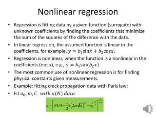
Nonlinear Regression Models • yt = ρyt-1 + xtβ - ρxt-1β + νt • Violates the assumption of the CRM as yt is a nonlinear function of parameters, ρ and β • i.e., the product • What does this mean for the use of Least Squares? • Would like to develop methods to obtain unbiased (and efficient) estimates of ρ and β
Nonlinear Regression Models • What if we specify the Cobb-Douglas production function via the following: • This cannot be transformed into linear model as we cannot take the natural log of both sides to linearize • No. of parameters = 3 (α, β1β2) • No. of regressors = 2 (L, K) • Again, we would like to develop an estimation algorithm that would allow us to obtain parameter estimates
Nonlinear Regression Models • Even though the above Cobb-Douglas specification is non-linear with respect to unknown regression coefficients, we can still use the principle of minimizing the sum of squared errors (SSE) to obtain parameter estimates where • SSE ≡ e′ewhere e is (T x 1) 5
Nonlinear Regression Models • Def. of a nonlinear regression model: A nonlinear regression model is one for which the 1st order conditions (FOC) for least squares estimation of the parameters are nonlinear functions of the parameters • Lets take a look at the FOC’s for minimizing the SSE under the general nonlinear model • Before we do this lets state some assumptions necessary for us to develop these FOC’s 6
Nonlinear Regression Models • Assumptions of the Nonlinear Regression Model • E(yt|Xt) = f(Xt,b) • f(.) is a non-linear (in parameters) twice continuously differentiable function • Model parameters are identifiable • Under the linear model this was the full rank assumption • There is no nonzero parameter vector β0 ≠ β such that f(Xt,β0) = f(Xt,β) general function
Nonlinear Regression Models • Assumptions of the Nonlinear Regression Model • With yt=f(Xt,β) + et we have E[et|f(Xt,β)] = 0→the error term is uncorrelated with the conditional mean function f(•) for all observations • Initially we assume that the et’s are identically and independently distributed (iid) • E[e2t|f(Xt,β), t=1,…,T] = σ2 • E[eiej|f(Xi,β),f(Xj,β)] = 0, j≠i, j,i=1,…,T • We will relax this assumption later • The distribution of Xt is independent of the distribution of et • The above implies: nonlinear function No t subscript
Nonlinear Regression Models • General Model Summary • yt = f(xt,b) + et • f(.) is non-linear (in parameters) differentiable function • et~(0,s2) • Need to optimize some type of objective function to obtain parameter estimates • Sum of squared errors (Nonlinear Least Squares Method, NLS) • Likelihood function (→Maximum Likelihood methods, ML) which we will review in the next section Notice no assumed distribution function
The Classical Regression Model • Lets review the Least Squares rule under the linear model: y=Xβ + e • y = β0 + β1X • Suppose we have two different estimators that generate values for β0, β1 • Which estimator is “preferred” ? 10
The Classical Regression Model • Given the above data and theoretical model we need to obtain parameter estimates to place the mean expenditure line in expenditure/income (X) space • Would expect the position of the line to be in the middleof the data points • What do we mean by middleas some et’s are positive and others negative • We need to develop some rule to locate this line 11
The Classical Regression Model • Least Squares Estimation rule • Chose a line (or plane) such that the sum of the squares of the vertical distances from each data point to the line defined by the coefficients (SSE) be as small as possible • The above line refers to E(yt)= Xtβ • SSE= Σtet2= Σt(yt-β0-β1xt)2 • Graphically, in the above scatter plot, the vertical distance from each point to the line representing the above linear relationship are the regression errors et E(yt|Xt)→conditional mean function 12
The Classical Regression Model • Let be an initial “guess” of the intercept and slope coefficients negative of initial conditional mean “guess” initial error term “guess” 13
The Classical Regression Model y3 yt y’s conditonal mean|β’s X3 y4 X4 Xt 14
The Classical Regression Model • Note that the SSE’s can be obtained via the following: SSE= e'e (Tx1) (1xT) (1x1) 15
The Classical Regression Model Naïve Model Xt has no effect on yt y3 yt y4 Xt • For the CRM least squares estimation rule we choose β0 and β1 to minimize the error sum of squares (SSE) 16
The Classical Regression Model • From the FOC for the minimization of the sum of squared errors (SSE) for the linear CRM model we have: • Can we be assured that whatever values of β0 and β1 we choose, they do indeed minimize the SSE? (i.e. only rely on FOC’s for estimation) (2 x 2) (2 x T) (2 x 1) Estimated value (1 x 1) 17
The Classical Regression Model • Can we be assured that whatever values of β0 and β1 we choose, they do indeed minimize the SSE? • Is the SSE function convex (vs concave) wrt β’s? 18
The Classical Regression Model Note: (Xβ)′=β′X′ Greene, p.949 • SSE=(y-Xβ)′(y-Xβ)= y′y - 2β′X′y + β′X′Xβ where X is (T x K), y is (T x 1) and β is (K x 1) • Focusing on dimensions: • y′y is (1 x T)(T x 1) = a (1 x 1) • β′X′y is (1 x K)(K x T)(T x 1) = a (1 x 1) matrix • β′X′Xβ is (1 x K)(K x T)(T x K)(K x 1) = a (1 x 1) matrix • Can we be assured that the SSE function is convex not concave wrt β’s? • Need to look at curvature conditions (1 x 1) 19
The Classical Regression Model • The matrix of second derivatives of SSE with respect to β0 and β1 can be shown to be: when first column of X is a vector of 1’s • HSSE must be positive definite for convexity of the SSE function • To be positive definite, every principle minor of HSSE needs to be positive 20
The Classical Regression Model • The two diagonal elements must be positive given the independence of ordering: In the above they are > 0 • |HSSE| is positive unless all values of x2 are 0 or 1 • →HSSE is positive definite • → SSE convex wrtβ’s under linear model 21
Nonlinear Regression Models • Now lets use the lessons learned from the CRM and applied to the nonlinear regression model: yt=f(Xt,β) + et • Nonlinear Least Squares (NLS) Method • Objective function is to minimize sum of squared errors (S) where S=e'e • e = y − f(X,β) • Normal equations of nonlinear model (i.e., FOC’s) are nonlinear in parameters • The solution to the FOC’s may be difficult and problem specific • In contrast to the Classical Regression Model (CRM) where βs=(X′X)-1X′y for all models e is (T x 1)
Nonlinear Regression Models • Nonlinear Least Squares Method • There is the possibility of more than one set of estimates that will satisfy the equation dS/dβ=0 • There could be both convex and concave regions of S • Could have local minimums and/or maximums • Given identification assumption these different parameters do not generate the same f(•) value even though dS/dβ=0 for the different parameter vectors 23
Nonlinear Regression Models (K*x 1) (K x 1) • yt=f(xt,β) + et et~iid(0,σ2) • With an estimate of β we obtain a predicted value of y cond. on that value: • With S(β) = e′e, the K-FOC’s for its minimization are via the chain rule: [y-f(X,β)]′[y-f(X,β)] (1 x 1) et divide through by -2 (1 x 1) divide through by -2
Nonlinear Regression Models • yt=f(xt,β) + et et~iid(0,σ2) • The K-FOC’s for minimizing the SSE’s
Nonlinear Regression Models • Assume we have the Cobb-Douglas production function we talked about earlier: • The partial derivatives are • The associated 3 FOC’s for minimizing the SSE can be represented via the following: Remember we are taking derivatives wrtcoefficeints
Nonlinear Regression Models • FOC: • Note that unlike the CRM with an intercept, because the above does not have an intercept, none of these FOC’s correspond to the condition: →residuals do no necessarily sum to 0 et
Nonlinear Regression Models • Nonlinear least squares estimate of β (βNL): • βNL minimizes the sum of square errors from the nonlinear function • Example of a quadratic function (wrt one parameter) • yt = βXt1 + β2Xt2 + et • Note we have two regressors and only 1 parameter → a single FOC 1 parameter, 2 X’s
Nonlinear Regression Models • The FOC to minimize S(β) is: Cubic function of β → 3 possible values of βNL
Nonlinear Regression Models • Given the above S(β) and FOC: Yt = βXt1 + β2Xt2 + et Lets apply the above model using the following data obtained from JHGLL, Ch. 12, Table 12.1 →
Nonlinear Regression Models Yt = βXt1 + β2Xt2 + et S(β)=e'e -0.9776→local maximum -2.0295→local minimum 1.1612→global minimum S(β) under alternative parameter values dS(β)/dβ=0
Nonlinear Regression Models • Nonlinear Least Squares Method • Unlike the CRM model we need to use specialized algorithms (methods) to minimize the SSE’s • Gauss-Newton (GN) • Newton-Raphson (NR) • Similar to ML algorithms we will review later • Similar to the CRM, use of NLS methods for parameter estimation does not require specific assumptions concerning error term distribution • i.e., do not need to assume the ε’s are normally distributed
Nonlinear Regression Models • To give you a sense of these algorithms assume we have the nonlinear regression model: yt = f(Xt, β) + εt • From Greene (p.288-289), the GN solution algorithm is based on the linear (First Order) Taylor series approximation to f(·) at a given parameter vector β0: • β0 is given • f(X,β0) is known • We want to evaluate f(X,β) • Lets assume we have a single parameter Initial value Change in β’s A parameter vector different from β0
Nonlinear Regression Models • For a single parameter we have • The slope of f(Xt,β) at point A is df(Xt,β)/dβ|β0=CB/BA (tangent slope at β0) • We can approximate this slope via: df(Xt,β)/dβ|β0≈[f(Xt,β)- f(Xt,β0)]/(β-β0) = DB/BA DB=f(Xt,β)- f(Xt,β0) BA= β-β0 f(Xt,β*) Functions evaluated at 2 parameter values f(•) D f(Xt,β) C A B f(Xt,β0) Approximate Slope = DB/BA β0 β
Nonlinear Regression Models Current estimate • From above figure df(Xt,β)/dβ|β0≈[f(Xt,β)- f(Xt,β0)]/(β-β0) • Rearranging: • With a single parameter this is the first-order Taylor series approximation to f(X,β) stated earlier initial parameter value → previous function value change in parameter value new function value
Nonlinear Regression Models • Extending this to multiple parameters where β is now of dimension K: • This implies • Placing known terms (given β0) on the LHS and defining y0: ε0 contains both true disturbance term ε and approx. error given the “≈” above. y=f(X,β)+ε May be a function of all K parameters unknown value T x K pseudo-regression new dep. variable
Nonlinear Regression Models yt = f(Xt, β) + εt Pseudo-regression: y0=Z0β+ε0 • That is: • The above results imply that for a given value of our coefficient vector, β0 • One can compute y0 and Z0 • Estimate the above pseudo-regression, y0= Z0β + ε0 using the CRM. “true” unknown error Function Approximation Error Dep. Variable Exog. Variable Referred to as Gauss-Newton Algorithm Remember Z0are K partial derivatives wrt the β’s evaluated at your current value of β, β0 , known at estimation time and is (T x K)
Nonlinear Regression Models • Lets look at the example given in Greene, p. 288 f 0
Nonlinear Regression Models • y0used as a dependent variable and regressed on the vectors Z10, Z20 and Z30 to give us estimates of β1, β2, and β3 • y0 = Z10β1 + Z20β2 + Z30β3 • Given the vector, β0, the Z0’s are predetermined like our traditional X’s 39
Nonlinear Regression Models Nonlinear Least Squares Algorithm (GN) yt=f(Xt,β) + εt Generate Initial Guess for , * Approx. f(Xt,) by First-Order Taylor Series Around * Update Estimate of to ** By Applying CRM to a Linear Pseudo Model GN Algorithm β* = β** No Check Optimality of S() (e.g. global minimum?) Yes y0= Z0β**+ ε0 β**=(Z0ʹZ0)-1 Z0ʹy0 Finished
Nonlinear Regression Models • Lets start with a single parameter model • Even though we have a single parameter, there could be multiple exogenous variables • Gauss-Newton Algorithm (in words) • We begin with an initial guess of β, β1 and approx. the function f(Xt,β) by a first-order Taylor Series around β1 • A 2nd value (guess) of β can be found by applying the CRM to a new linear model, the linear pseudo-model. • By repeatedly applying the formula (as in iteration n+1) until convergence occurs, we will have reached a point that is a solution to the FOC for minimizing the SSE’s.
Nonlinear Regression Models • Gauss-Newton Algorithm • Single Parameter Model: yt=f(xt,β) + εt • Residual Sum of Squares: • FOC for Minimum: ε′Z(β) = 0
Nonlinear Regression Models • Gauss-Newton Algorithm • As noted above, the First-Order Taylor Series Approximation to f(Xt,β) is: • Substituting this into S(β): Let β1 be the initial value ≡Zt(β1) et = yt - f(xt,β) S(β)=e′e New β value β1 already known → , Zt known
Nonlinear Regression Models • Gauss-Newton Algorithm • Linearpseudo-regression model: Given we know β1, this is known “Y” “X” Given the value of β1, “Y” and “X” are predetermined (known) • Single Parameter Model: yt = f(xt,β) + εt • S(β)=ε′ε
Nonlinear Regression Models • Gauss-Newton Algorithm • Linearpseudo-model: For iteration 1, β1 is known New “Error” New Estimate “(X'X)-1” “X'Y”
Nonlinear Regression Models • Gauss-Newton Algorithm • Note: ith subscript refers to iteration number notith parameter New “Error” For iteration 2, β2 is known
Nonlinear Regression Models • Gauss-Newton Algorithm • Residual Sum of Squares at the nth iteration: • If βn generates a minimum S(βn): • For optimality: Does ε(βn)′Z(βn) = 0? εt(βn) Zt(βn) 47
Nonlinear Regression Models • Gauss-Newton Algorithm • Optimality: Does ε(βn)′Z(βn) = 0? • How close to 0 is the above? • In reality the above sum will likely never be exactly equal to 0 • You need to make a judgment as to how close is close enough • Can evaluate closeness in terms of changes in S(β) across iterations • Need to adjust for scale (i.e., % change across iterations) • Can evaluate closenessin terms of changes in β’s across iterations • Need to adjust for scale (i.e., max. absolute % change of any coefficient across iterations) 48
Nonlinear Regression Models • Gauss-Newton Algorithm • Linear pseudo-model: Previous Estimate Previous Estimate IterationStep Full Gauss-Newton Iteration
Nonlinear Regression Models • Gauss-Newton Algorithm • From the above we have Iteration Step With Z′Z being the sum of squares of slope of f(X,βn). Remember we are minimizing S(β). Given definition of Z(βn), this is FOC for minimizing non-linear sum of squared errors we derived earlier 50