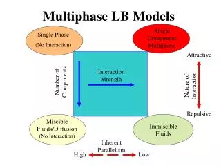
Multicomponent Multiphase LB Models
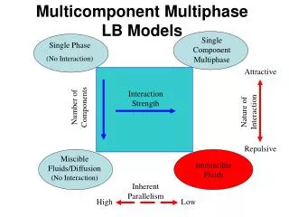
Multicomponent Multiphase LB Models. Single Component Multiphase. Single Phase (No Interaction). Attractive. Interaction Strength. Number of Components. Nature of Interaction. Multi- Component Multiphase. Repulsive. Miscible Fluids/Diffusion (No Interaction). Immiscible Fluids.

Multicomponent Multiphase LB Models
E N D
Presentation Transcript
Multicomponent Multiphase LB Models Single Component Multiphase Single Phase (No Interaction) Attractive Interaction Strength Number of Components Nature of Interaction Multi- Component Multiphase Repulsive Miscible Fluids/Diffusion (No Interaction) Immiscible Fluids Inherent Parallelism High Low
Often just need another loop: for( subs=0; subs<NUM_FLUID_COMPONENTS; subs++) for( j=0; j<LY; j++) for( i=0; i<LX; i++) { … } Adding a component/substance
// Compute density, Eq. (97), and the sums used (below) // in the velocities. for( subs=0; subs<NUM_FLUID_COMPONENTS; subs++) for( j=0; j<LY; j++) for( i=0; i<LX; i++) { rhoij[subs] = 0.; u_xij[subs] = 0.; u_yij[subs] = 0.; if( !is_solid_node[j][i]) { for( a=0; a<9; a++) { rhoij[subs] += ftemp_ij[a]; u_xij[subs] += ex[a]*ftemp_ij[a]; u_yij[subs] += ey[a]*ftemp_ij[a]; } } } One composite u for feq calculation(Eqn. 95 in Sukop and Thorne; note error in 2006 printing)
// Compute the composite velocity and individual velocities. for( j=0; j<LY; j++) { for( i=0; i<LX; i++) { if( !is_solid_node[j][i]) { ux_sum = u_xij[0]/tau0 + u_xij[1]/tau1; uy_sum = u_yij[0]/tau0 + u_yij[1]/tau1; if( rhoij[0] + rhoij[1] != 0) { // Composite velocity, Eq. (95). uprime_x = ( ux_sum) / ( rhoij[0]/tau0 + rhoij[1]/tau1); uprime_y = ( uy_sum) / ( rhoij[0]/tau0 + rhoij[1]/tau1); } else { uprime_x = 0.; uprime_y = 0.; } // Individual velocities, Eq. (96), x-direction. if( rhoij[0] != 0) { u_xij[0] = u_xij[0] / rhoij[0]; } else { u_xij[0] = 0.; } if( rhoij[1] != 0) { u_xij[1] = u_xij[1] / rhoij[1]; } else { u_xij[1] = 0.; } // Individual velocities, Eq. (96), y-direction. if( rhoij[0] != 0) { u_yij[0] = u_yij[0] / rhoij[0]; } else { u_yij[0] = 0.; } if( rhoij[1] != 0) { u_yij[1] = u_yij[1] / rhoij[1]; } else { u_yij[1] = 0.; } } } } One composite u for feq calculation
Interparticle Forces • // Compute fluid-fluid interaction force, equation (98), • // (assuming periodic domain). • // • // We begin by computing psi even though in this implementation • // it is the same as rho. A different function of rho could • // be substituted here. • for( subs=0; subs<NUM_FLUID_COMPONENTS; subs++) • for( j=0; j<LY; j++) • for( i=0; i<LX; i++) • if( !is_solid_node[j][i]) • { • psi[subs][j][i] = rho[subs][j][i]; • }
Interparticle Forces • // Compute the summations in Eq. (98). • for( subs=0; subs<NUM_FLUID_COMPONENTS; subs++) • { • for( j=0; j<LY; j++) • { • jp = ( j<LY-1)?( j+1):( 0 ); • jn = ( j>0 )?( j-1):( LY-1); • for( i=0; i<LX; i++) • { • ip = ( i<LX-1)?( i+1):( 0 ); • in = ( i>0 )?( i-1):( LX-1); • Fxtemp = 0.; • Fytemp = 0.;
Interparticle Forces • if( !is_solid_node[j][i]) • { • if( !is_solid_node[j ][ip]) // neighbor 1 • { Fxtemp = Fxtemp + WM*ex[1]*psi[subs][j ][ip]; • Fytemp = Fytemp + WM*ey[1]*psi[subs][j ][ip]; } • if( !is_solid_node[jp][i ]) // neighbor 2 • { Fxtemp = Fxtemp + WM*ex[2]*psi[subs][jp][i ]; • Fytemp = Fytemp + WM*ey[2]*psi[subs][jp][i ]; } • if( !is_solid_node[j ][in]) // neighbor 3 • { Fxtemp = Fxtemp + WM*ex[3]*psi[subs][j ][in]; • Fytemp = Fytemp + WM*ey[3]*psi[subs][j ][in]; } • if( !is_solid_node[jn][i ]) // neighbor 4 • { Fxtemp = Fxtemp + WM*ex[4]*psi[subs][jn][i ]; • Fytemp = Fytemp + WM*ey[4]*psi[subs][jn][i ]; } • if( !is_solid_node[jp][ip]) // neighbor 5 • { Fxtemp = Fxtemp + WD*ex[5]*psi[subs][jp][ip]; • Fytemp = Fytemp + WD*ey[5]*psi[subs][jp][ip]; } • if( !is_solid_node[jp][in]) // neighbor 6 • { Fxtemp = Fxtemp + WD*ex[6]*psi[subs][jp][in]; • Fytemp = Fytemp + WD*ey[6]*psi[subs][jp][in]; } • if( !is_solid_node[jn][in]) // neighbor 7 • { Fxtemp = Fxtemp + WD*ex[7]*psi[subs][jn][in]; • Fytemp = Fytemp + WD*ey[7]*psi[subs][jn][in]; } • if( !is_solid_node[jn][ip]) // neighbor 8 • { Fxtemp = Fxtemp + WD*ex[8]*psi[subs][jn][ip]; • Fytemp = Fytemp + WD*ey[8]*psi[subs][jn][ip]; } • } /* if( !is_solid_node[j][i]) */
Interparticle Forces • Fx[subs][j][i] = Fxtemp; • Fy[subs][j][i] = Fytemp; • } /* for( i=0; i<LX; i++) */ • } /* for( j=0; j<LY; j++) */ • } /* for( subs=0; subs<NUM_FLUID_COMPONENTS; subs++) */ • // Compute the final interaction forces of Eq. (98) using • // the summations computed above. • for( j=0; j<LY; j++) • { • for( i=0; i<LX; i++) • { • if( !is_solid_node[j][i]) • { • Fxtemp = Fx[1][j][i]; • Fx[1][j][i] = -G*psi[1][j][i]*Fx[0][j][i]; • Fx[0][j][i] = -G*psi[0][j][i]*Fxtemp; • Fytemp = Fy[1][j][i]; • Fy[1][j][i] = -G*psi[1][j][i]*Fy[0][j][i]; • Fy[0][j][i] = -G*psi[0][j][i]*Fytemp; • } • } • }
Complementary Densities • 6,000 ts Domain 5X100 Periodic boundary
Complementary Densities • 2,500 ts Domain 100X100 Periodic boundary
#define BIG_U_X( u_, rho_) \ (u_) \ + lattice->param.tau[subs] \ * lattice->force[subs][n].force[0]/(rho_) \ + lattice->param.tau[subs] \ * lattice->force[subs][n].sforce[0]/(rho_) \ + lattice->param.tau[subs] \ * lattice->param.gforce[subs][0] #define BIG_U_Y( u_, rho_) \ (u_) \ + lattice->param.tau[subs] \ * lattice->force[subs][n].force[1]/(rho_) \ + lattice->param.tau[subs] \ * lattice->force[subs][n].sforce[1]/(rho_) \ + lattice->param.tau[subs] \ * lattice->param.gforce[subs][1] Computing big U (aka ueq)
Multicomponent Multiphase LBM • Separate distributions • Repulsive interaction
Laplace Law • Interfacial tension (as opposed to surface tension between a liquid and its own vapor)
MCMP LBM with Surfaces • Like SCMP except each fluid phase can interact with surface • Two surface interaction parameters, one fluid/fluid • Young’s Equation:
MCMP SForce • for( j=0; j<LY; j++) • { • jp = ( j<LY-1)?( j+1):( 0 ); • jn = ( j>0 )?( j-1):( LY-1); • for( i=0; i<LX; i++) • { • ip = ( i<LX-1)?( i+1):( 0 ); • in = ( i>0 )?( i-1):( LX-1); • if( !is_solid_node[j][i]) • { • sum_x=0.; • sum_y=0.; • if( is_solid_node[j ][ip]) // neighbor 1 • { sum_x = sum_x + WM*ex[1]; • sum_y = sum_y + WM*ey[1];} • if( is_solid_node[jp][i ]) // neighbor 2 • { sum_x = sum_x + WM*ex[2]; • sum_y = sum_y + WM*ey[2];} • if( is_solid_node[j ][in]) // neighbor 3 • { sum_x = sum_x + WM*ex[3]; • sum_y = sum_y + WM*ey[3];} • if( is_solid_node[jn][i ]) // neighbor 4 • { sum_x = sum_x + WM*ex[4]; • sum_y = sum_y + WM*ey[4];} • if( is_solid_node[jp][ip]) // neighbor 5 • { sum_x = sum_x + WD*ex[5]; • sum_y = sum_y + WD*ey[5];} • if( is_solid_node[jp][in]) // neighbor 6 • { sum_x = sum_x + WD*ex[6]; • sum_y = sum_y + WD*ey[6];} • if( is_solid_node[jn][in]) // neighbor 7 • { sum_x = sum_x + WD*ex[7]; • sum_y = sum_y + WD*ey[7];} • if( is_solid_node[jn][ip]) // neighbor 8 • { sum_x = sum_x + WD*ex[8]; • sum_y = sum_y + WD*ey[8];} • for( subs=0; subs<NUM_FLUID_COMPONENTS; subs++) • { • sforce_x[subs][j][i] = -Gads[subs]*sum_x; • sforce_y[subs][j][i] = -Gads[subs]*sum_y; • } • } • } • }
MCMP surface forces • A surrounded by itself: • FA = GrArB • A surrounded by solid: • FadsA = GadsArA • FadsA =FAleads to: • Since complimentary density is low, Gads should be small relative to G
90-degree contact angle Multicomponent fluids interacting with a surface when G = 0.1and Gads1 = Gads2 = -0.01.
45° Contact Angle Wetting fluid must have lowest Gads Multicomponent fluids interacting with a surface when G = 0.1, Gads1 = -0.02, and Gads2 = 0.0507.
q1 u2 H-h q2 u1 h Y b Z g 2 Phase Flow Analytical Solution
Countercurrent air and water Pressure gradient in air phase Pressure gradient in water phase
Density and Viscosity Contrasts • Large density and viscosity contrasts are a major challenge of LBM research. • McCracken and Abraham (2005): pressure in standard multicomponent LB models is p = (r1 + r2)cs2, where cs is the speed of sound • Significance is that for total pressure to be constant, the sum of the densities of the 2 species must be constant • Not the case in real gasses, where differing molecular weights lead to constant pressures despite different densities